Plotting Curvilinear Squares for Electromagnetic Fields
•Download as DOCX, PDF•
2 likes•1,258 views

This document describes a laboratory experiment conducted by a student to plot electric and displacement fields using the curvilinear square method for different conductor configurations. In the first part, equipotential lines and flux lines were drawn between two conductors set to 0-60V. The electric field intensity was calculated. In the second part, the capacitance of a coaxial capacitor was calculated theoretically and by plotting field lines, yielding similar results within human and method errors. The purpose of plotting fields graphically and comparing calculations to theory was achieved.

Recommended
More Related Content
What's hot
What's hot (20)
Similar to Plotting Curvilinear Squares for Electromagnetic Fields
Similar to Plotting Curvilinear Squares for Electromagnetic Fields (20)
Recently uploaded
Recently uploaded (20)
Plotting Curvilinear Squares for Electromagnetic Fields
- 1. UNIVERSITY OF BOTSWANA FACULTY OF ENGINEERING AND TECHNOLOGY DEPARTMENT OF ELECTRICAL ENGINEERING LAB 1: FIELD PLOTTING CURVILINEAR SQUARES ELECTROMAGNETIC FIELD THEORY EEB 327 AUTHOR: NTSHOLE B.T 201301848 GROUP B2 DATE OF SUBMISSION: 11/03/2016
- 2. ABSRACT The intension of this experiment was to plot E and D for a given configuration of conductor boundaries using graphical field plotting method known as the curvilinear method. Equipotential lines and flux lines were drawn at 90degrees keeping the potential difference (Pd) between the equipotential lines constant. In the second part of the experiment, the potentials at the conductor boundaries were distinct to be 0 to 60V and the region between the conductor boundaries was assumed to be filled with air. The magnitude of electric field intensity was calculated using the following formula for 2mm of radius provided. The formula that was used most of the times to calculate the estimated electrical field is given below; 𝐸 = ∆𝑉 ∆𝐿 𝑁 It was found out that practical and theoretical results were similar, but there were slight deviations from actual results due to the human errors when plotting as well as insufficient space for plotting field lines.
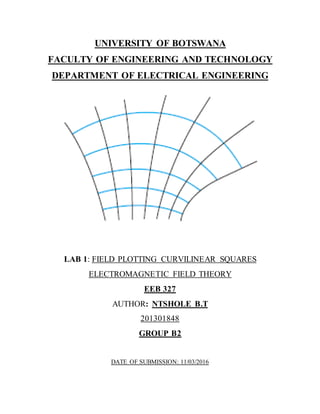
- 3. INTRODUTION The main objective was to use a graphical field plotting technique to plot an E and D field for a given configuration of conductor boundaries. Considering the curvilinear method; Curvilinear method The procedure was based on the following facts: A conductor boundary was an equipotential surface, The electric field intensity and electric flux density were both perpendicular to the equipotential surfaces E and D were perpendicular to the conductor boundaries and possess zero tangential values The lines of electric flux begun and terminated on the charge which resulted in a charge- free homogenous dielectric which begun and terminated only on the conductor boundaries. The implications of these statements were considered by drawing streamlines on the sketch showing equipotential surfaces. Figure 1: (a) Sketch of the equipotential surfaces between two conductors. The increment of potential between each of the two adjacent equipotentials is the same.(b) One flux line has been drawn from A to A_, and a second from B to B_. Source: [1] H.Hayt, W. (n.d.). Engineering Electromagnetics, page155. In Figure 1 above, two conductor boundaries are shown and equipotentials were drawn with a constant potential difference between the lines. These lines were only the cross sections of the equipotential surfaces which are cylinders. No variations in the direction normal to the surface of the paper were permitted. The streamline to begin, or flux line, at A on the surface of the more positive conductor were arbitrarily chosen. It leaves the surface normally and crossed at right angles the undrawn but very real equipotential surfaces between the conductor and the first surface shown. The line is continued to the other conductor, obeying the single rule that the intersection with each equipotential must be square.
- 4. RESULTS ( 𝑎) 𝐶𝑎𝑝𝑎𝑐𝑖𝑡𝑎𝑛𝑐𝑒 𝑝𝑒𝑟 𝑚𝑒𝑡𝑒𝑟 𝑙𝑒𝑛𝑔𝑡ℎ 𝑓𝑜𝑟 𝑓𝑖𝑔𝑢𝑟𝑒 2 𝐶 = 8.854 × 10−12 × 14 3 𝐶 = 41.3187𝑝𝐹 ( 𝑏) 𝐸 𝑎𝑡 𝑡ℎ𝑒 𝑙𝑒𝑓𝑡 𝑠𝑖𝑑𝑒 𝑜𝑓 𝑡ℎ𝑒 60𝑉 𝑐𝑜𝑛𝑑𝑢𝑐𝑡𝑜𝑟 𝑖𝑓 𝑖𝑡𝑠 𝑡𝑟𝑢𝑒 𝑟𝑎𝑑𝑖𝑢𝑠 𝑖𝑠 2𝑚𝑚 𝐸 = ∆𝑉 ∆𝐿 𝑁 𝐸 = (60 − 0) 2 × 10⁻³ 𝐸 = 30𝐾𝑉 𝑚 ( 𝑐) 𝜌𝑠 𝑎𝑡 𝑡ℎ𝑎𝑡 𝑝𝑜𝑖𝑛𝑡 𝜌𝑠 = 𝜀𝐸 𝜌𝑠 = 8.854 × 10−12 × 30 × 103 𝜌𝑠 = 265𝑛𝐶 𝑚2
- 5. 𝑐𝑜𝑎𝑥𝑖𝑎𝑙 𝑐𝑎𝑝𝑎𝑐𝑖𝑡𝑜𝑟 𝑇ℎ𝑒𝑜𝑟𝑒𝑡𝑖𝑐𝑎𝑙 𝐶 = 2𝜋𝜖 𝑂 𝑙𝑛 𝑎 𝑏 𝑤ℎ𝑒𝑟𝑒 𝑎 = 8𝑐𝑚 𝑎𝑛𝑑 𝑏 = 2.5𝑐𝑚 𝑎𝑟𝑒 𝑡ℎ𝑒 𝑡𝑤𝑜 𝑟𝑎𝑑𝑖𝑖 𝑜𝑓 𝑡ℎ𝑒 𝑐𝑖𝑟𝑐𝑙𝑒𝑠 𝐶 = 2 × 𝜋 × 8.854 × 10⁻¹² 𝑙𝑛 8 2.5 𝐶 = 47.828𝑝𝐹 𝑃𝑟𝑎𝑐𝑡𝑖𝑐𝑎𝑙 𝐶𝑎𝑝𝑎𝑐𝑖𝑡𝑎𝑛𝑐𝑒 𝑐𝑎𝑙𝑐𝑢𝑙𝑎𝑡𝑒𝑑 𝑓𝑟𝑜𝑚 𝑡ℎ𝑒 𝑑𝑟𝑎𝑤𝑖𝑛𝑔 𝐶 = 𝜖 𝑂 𝑁 𝑄 𝑁 𝑉 𝐶 = 8.854 × 10⁻¹² × ( 360 12 ) 5 𝐶 = 53.124𝑝𝐹
- 6. DISCUSSION Both theoretical and practical results were not that much different because this approach lacks the accuracy of more elegant methods, allows fairly quick estimates of capacitance while providing a useful visualization of the field configuration. The curvilinear square method required patience and skill which the writer used to his advantage to get accurate results. The slight deviation in the results was because of the following reasons: insufficient practice on plotting the equipotential lines and flux lines, Human error when plotting Failing to terminate most field lines and equipotential lines not crossing over them by 90 degrees. CONCLUSION The purpose of this experiment was achieved which was to plot E and D for a given configuration of conductor boundaries. It was accomplished because results generated in this report satisfy the objective of this experiment. The capacitance calculated from the drawing was found to be 𝟓𝟑. 𝟏𝟐𝟒𝒑𝑭 that wasn’t different from the theoretical capacitance which was found to be𝟒𝟕. 𝟖𝟐𝟖𝒑𝑭. The capacitance per meter length for figure 2 (on appendices) obtained was not accurate because the author had human errors mostly on field lines not making 90 degrees with the equipotential lines hence the capacitance per length was affected and was found to be 𝟒𝟏. 𝟑𝟏𝟖𝟕𝒑𝑭. REFFERENCES - H.Hayt, W. (n.d.). Engineering Electromagnetics, pages 162 to 168 - Essential electromagnetism.(pdf), pages 74-77.