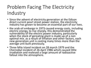
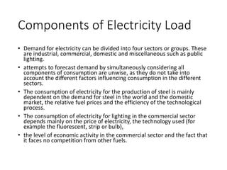
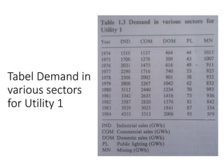
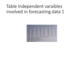
Summary of Modern power system planning part one "The Forecasting of Growth of Demand for Electrical Energy" the main topic of this chapter is the analysis of the various techniques required for utility planning engineers to optimally plan the expansion of the electrical power system.

1. Modern Power System
Planning
Chapter One
The Forecasting of Growth of Demand for Electrical
Energy
• X.Wang and J.R McDonald
• MarcelinoMadrigal, Ph.D
Sr. Energy Specialist,
Sustainable Energy Department, The World Bank
• https://www.slideshare.net/linsstalex?utm_campaign=profiletracking&utm_medium=sssite&utm_source=ssslideview

2. Problem
Facing
The
Electricity
Industry
Since the advent of electricity generation at the
Edison direct current pearl street power station,
the electricity industry has grown to become an
essential part of our lives.
the arab oil embargo in 1973 caused energy costs,
including electric energy, to rise sharply. this
demonstrated the vulnerability of the electric
power industry, particularly when the stock of
gereating plant is made up of a non optimal mix.
as a result of inflation and other factors, each new
generation unit is costing many times more than
the average unit built previously.
Three Mile Island incident on 28 march 1979 and
the Chernobyl incident of 26 April 1986 which
caused little irradiation and realesed a large
amount of radioactive fallout into the
atmosphere.

3. Technology
Options
Available to
The Electricity
industry
• Electricity industries must also consider
alternatives available at both ends of the
electricity system, i.e. the supply and
demand sides.
• some of the technologies available are
renewable energy sources and energy
storage systems for the supply side. Option
on the demand side are energy
management and conservation strategies.
• load management has been developed in
order to improve operational and economic
efficiencies in the supply of electric energy.
The primary purpose of these schemes is to
change the electricity usage patterns by
exerting control on the load so that demand
for electrical energy can be shifted from
peak to off peak periods.

4. • Demand for electricity can be controlled at these peak times
by employing either indirect or direct control techniques.
• Indirect load control strategies involve controlling demand by
the use of multi block time of day tariffs, spot pricing and
special off-peak rates.
• other demand side option available are programmes of
improving the efficiency of user appliances. Such techniques
are also known as the end use efficiency option, which is
another form of conserving energy.
• Energy conservation options are attractive because they are
less experience to implement than building additional
generating capacities. furthermore, there is no long lead time
associated with their application.

5. The Corporate Planning Process
1. The need forecasts in The Electricity Industry
Forecasting plays an important role in the electric power industries. Time
scales for which it is necessary to have forecasts of electricity consumption
and demand fall into three groups: the long term for the period covering
seven years onwards; the short to medium term for the period covering up to
seven years; the sort term which covers the time-scale of up to one day ahead.
2. Long-term forecasting and uncertainties
Forecasting the future needs for electricity is a difficult task at the best of
times. Projects are large and lead times are long, larger projects like building a
nuclear power plant can take at least fourteen years of planning and
construction before generation can be started. This generation period may
become longer in the future, especially as safety and conservation measures
become more stringent.

6. 3. Decision-Making process
The multiple scenario methods produce a large number of
“futures”. Planners should determine their plan of actions based
on what future they favour or perhaps on futures that they feel
will probably come true. In determining the plan of actions,
utilities are forced to take into account concerns and challenge of
the society that they serve.

7. the scope
of the
chapter
• The first part of this chapter is concerned
with methods of long-term forecasting
• Load management and conservation
measures are two demand side options that
allow a utility to control load growth as well
as improving system performance. Another
part of this work will be to develop models
that allow the effects of these strategic
actions to be taken into account
• The models integrate both the engineering
and econometric approaches and therefore
are able to make a realistic assessment of
the contribution that changes in appliance
efficiency have on electric savings.

8. Long-term forecasting
Techniques
• Load forecasting has always been an integral part power system planning and
operation.
• The many types of forecasting procedures can be classified into five broad
categories: subjective, univariate, multivariate, end user and combination.
• Using the subjective approach, forecast can be made on a subjective basis
using judgement, intuition, commercial knowledge and any other relevant
information
• Univariate forecast are based entirely on past observation in a given time
series
• Multivariate forecasts, on the other hand attempt to establish casual or
explanatory relationships. Multivariate models are sometimes called “casual”
or ‘prediction’ models.

9. • Forecasting can be made by directly specifying those
activities that give rise to sale or consumption of
electricity demand. This method, which is called the end
user approach
• In practice different techniques are used in combination
to produce new an in many cases better forecasting
results. Such an approach can be made by amalgamating
two or more forecasts, following various combination
procedures.

10. Extrapolation of trend curves
1. Exponential Growth Curves
Exponential growth patterns appear frequently in practice and
correspond to a steady, constant growth rate.
An exponential curve is given by the equation
𝒀 𝒕 = 𝐞𝐱𝐩 𝒂 + 𝒃𝒕 ; (1.1)
𝑎 is a constant, 𝑏 represents the growth rate and 𝑡 is the time unit.
it becomes evident that the curve represents a straight line:
𝐥𝐧 𝒀 𝒕 = 𝒂 + 𝒃𝒕 ; (1.2)
In statistical term,
𝒀 𝒕 = 𝐞𝐱𝐩 𝒂 + 𝒃𝒕 + 𝜺 𝒕 ; (1.3)
𝐥𝐧 𝒀 𝒕 = 𝒂 + 𝒃𝒕 + 𝜺 𝒕
∗ ; (1.4)
Where 𝜺 𝒕 and 𝜺 𝒕
∗ represent error terms.

11. 2. Saturating Growth Curves
Some curves are characterized as having their slope
change from an increasing rate of growth to a decreasing
one. In general the nature of these curves exhibit the
following features:
• An initial period of relatively slow but gradually
increasing growth.
• An intermediate period of rapid growth
• This is followed by a final period where the rate of
growth declines and observed data appear to reach a
saturation level.

12. 3. Three-Point Method
Many estimation methods already exist in literature; a
least squares technique known as the gomes method is
given in Gregg and much simpler procedure, but just as
effective, is the three-point method in Gregg and
Yeomans.

13. Taking the mean values of each section as
𝑌1 = 𝑘 + 𝑎
𝑏0+𝑏1+𝑏2
𝑁
(1.5)
𝑌2 = 𝑘 + 𝑎
𝑏3+𝑏4+𝑏5
𝑁
(1.6)
𝑌3 = 𝑘 + 𝑎
𝑏6+𝑏7+𝑏8
𝑁
(1.7)
Where N is the total data each section
Solving the equation gives values of 𝑎, 𝑏 and 𝑘 as follows:
𝑏 =
𝑁 𝑌3−𝑌2
𝑌2−𝑌1
𝑎 =
𝑁(𝑌2−𝑌1)
𝑏3+𝑏4+𝑏5 −(𝑏0+𝑏1+𝑏2)
𝑘 = 𝑌1 − 𝑎
𝑏0+𝑏1+𝑏2
𝑁

14. Box-Jenkins Forecasting
Procedure
This forecasting procedure was developed by G.E.P.
Box and G.M Jenkins almost three decades ago, and
is still very popular among forecasters.
Box-Jenkins approach to time series model building
is a method of finding for a given set of data, an
autoregressive integrated moving average (ARIMA)
model that adequately represents the data
generating process.

15. 1. Autocorrelation
The autocorrelation among successive values of the data
is a key tool in identifying the best model that can
describe the data.
The concept of correlation between two variables is a
measure of the association between the two variables. It
describe what happens to one of the variables if there is a
change in the other.
2. Types of Box-Jenkins Model
The box-Jenkins methodology assumes three general
classes of model that can describe any type or pattern of
time series data.
• Autoregressive (AR) model
• The moving average (MA) model
• The autoregressive moving average (ARMA) model

16. An autoregressive model describes the current value of the process in
terms of a finite, linear aggregate of previous values of the process and a
perturbation 𝑎 𝑡.
If the values of the process at equally spaced times 𝑡, 𝑡 − 1, 𝑡 − 2, … are
𝑌𝑡, 𝑌𝑡−1, 𝑌𝑡−2, … , and assuming that ෩𝑌𝑡, ෨𝑌𝑡−1, … are their deviations form 𝜇,
a parameter that determines the ‘level’ of the process such that the
relationship
෨𝑌𝑡 = 𝑌𝑡 − 𝜇
Exists, then
𝑌𝑡 = ∅1 𝑌𝑡−1 + ∅2 𝑌𝑡−2 + ⋯ + ∅ 𝑝 𝑌𝑡−𝑝 + 𝑎 𝑡
Where ∅1,…, ∅ 𝑝 are the autoregressive parameters.
A moving average model assumes that the current value of the process
can be expressed as a finite number of previous error values, 𝑎. Thus the
model is expressed as
෨𝑌𝑡 = 𝑎 𝑡 − 𝜃1 𝑎 𝑡−1 + 𝜃2 𝑎 𝑡−2 − ⋯ − 𝜃 𝑞 𝑎 𝑡−𝑞
and is called a moving average process of order q, MA(q), where 𝜃1, …, 𝜃 𝑞
are the moving average parameters.

17. An autoregressive model describes the current value of the process in
terms of a finite, linear aggregate of previous values of the process and a
perturbation 𝑎 𝑡.
If the values of the process at equally spaced times 𝑡, 𝑡 − 1, 𝑡 − 2, … are
𝑌𝑡, 𝑌𝑡−1, 𝑌𝑡−2, … , and assuming that ෩𝑌𝑡, ෨𝑌𝑡−1, … are their deviations form 𝜇,
a parameter that determines the ‘level’ of the process such that the
relationship
෨𝑌𝑡 = 𝑌𝑡 − 𝜇
Exists, then
𝑌𝑡 = ∅1 𝑌𝑡−1 + ∅2 𝑌𝑡−2 + ⋯ + ∅ 𝑝 𝑌𝑡−𝑝 + 𝑎 𝑡
Where ∅1,…, ∅ 𝑝 are the autoregressive parameters.
Defining an autoregressive operator of order p by
∅ 𝐵 = 1 − ∅1 𝐵1
− ∅2 𝐵2
− ⋯ − ∅ 𝑝 𝐵 𝑝
Where 𝐵 is the backwards shift operator, such that 𝐵 𝑝
= 𝑎 𝑡−𝑝. The
autoregressive model may be expressed more succinctly as
∅ 𝐵 ෨𝑌𝑡 = 𝑎 𝑡

18. A moving average model assumes that the current value of the process
can be expressed as a finite number of previous error values, 𝑎. Thus the
model is expressed as
෨𝑌𝑡 = 𝑎 𝑡 − 𝜃1 𝑎 𝑡−1 + 𝜃2 𝑎 𝑡−2 − ⋯ − 𝜃 𝑞 𝑎 𝑡−𝑞
and is called a moving average process of order q, MA(q), where 𝜃1, …, 𝜃 𝑞
are the moving average parameters.
The third model considered by the Box-Jenkins approach is mixed model.
The model include both the autoregressive and moving average terms in
the model. This lead to a model describe by
෨𝑌𝑡 = ∅1
෨𝑌𝑡−1 + ⋯ + ∅ 𝑝
෨𝑌𝑡−𝑝 + 𝑎 𝑡 − 𝜃1 𝑎 𝑡−1 + 𝜃2 𝑎 𝑡−2 − ⋯ − 𝜃 𝑞 𝑎 𝑡−𝑞
Or the model can also be represented as
∅ 𝐵 ෨𝑌𝑡 = 𝜃(𝐵)𝑎 𝑡
Where
∅ 𝐵 = 1 − ∅1 𝐵1 − ∅2 𝐵2 − ⋯ − ∅ 𝑝 𝐵 𝑝
𝑝 = order of the autoregressive polynomial
𝜃 𝐵 = 1 − 𝜃1 𝐵1 − 𝜃2 𝐵2 − ⋯ − 𝜃 𝑝 𝐵 𝑝
𝑞 = order of the moving average polynomial

19. 3. Identifying an Appropriate model
Differencing process A non-stationary sequence can be
transformed into a stationary sequence by taking
successive differences of the series.
Identifying p and q Once stationarity is obtained, p and q
are identified by studying the patterns of the
autocorrelation and partial autocorrelation functions
generated.
4. Parameter EStimation
Once a model is identified, the parameters of the model
are estimated. To illustrate this process, consider an
ARIMA(1,2,1) model:
1 − ∅1 𝐵1 𝑤𝑡 = (1 − 𝜃1 𝐵1)𝑎 𝑡

20. 5. Diagnostic Checking
After the parameters in a model have been estimated, it is
necessary to check whether the model assumptions are
satisfied. The phase is called diagnostic checking. There
are two possible conclusions:
• The errors are random, which means that the fitted
model has eliminated all dependence from data and
what remains are random errors.
• The errors are not random and the fitted model has not
removed all of the dependency.
6. Forecasting Process
When a model has been identified, the parameters
estimated and the residuals shown to be random,
forecasting with the model is possible.
1 − ∅1 𝐵1 𝛻2 𝑌𝑡 = (1 − 𝜃1 𝐵1)𝑎 𝑡

21. Multivariate Procedures
The causal methods try to relate
electricity consumption to other
sets of explanatory variables.
Example of such methods are
regression and multiple regression
analysis.
Forecasting begins with the process
of determining the variables that
are to be taken into consideration.
These variables are assumed to
have an influence over the demand
for electricity.
hooke used the size household and
the number of customers to build a
model for domestic demand, while
the commercial and industrial
demands were projected with the
inclusion of the business index as
another exogenous variable.

22. • Stepwise Regression
Regression equation modelling is considered as the starting point for econometric
research.
The technique postulates the casual relationship between a dependent variable and
one or more independent variables. it attempts to explain observed changes in a
dependent variable caused by changes in the independent variables.
Stepwise regression starts by
• first calculating the correlation coefficients of all the variables; this includes the
dependent as well as the independent variables.
• The first variable to enter the regression is the variable that is most highly
correlated with the dependent variable.
• These two variables are regressed, and the least squares estimate is obtained.
• The variable with the highest partial correlation coefficient is then chosen to enter
the modal
• If the overall F-test shows that this new regression equation is significant, both
variables are retained and the search for the next variable to be included is
continued.
the final model must satisfy all criteria and pass all the tests used, in order to assess
the goodness of fit.

23. The
Scenarios
Method
The scenarios method
specifically tries to
conceive all possible
futures and explore the
path leading to them in
order to clarify present
actions and their possible
consequences.
1
The method comprises
two phases: the
construction of a
database and, on this
basis, the setting of
scenario that lead to the
generation of forecasts.
2
In conclusion, scenario
analysis can be useful in
considering the
uncertainties and future
developments associated
with future electricity
demand.
3

24. Components of Electricity Load
• Demand for electricity can be divided into four sectors or groups. These are
industrial, commercial, domestic and miscellaneous such as public lighting.
• attempts to forecast demand by simultaneously considering all components of
consumption are unwise, as they do not take into account the different factors
influencing consumption in the different sectors.
• The consumption of electricity for the production of steel is mainly dependent
on the demand for steel in the world and the domestic market, the relative fuel
prices and the efficiency of the technological process.
• The consumption of electricity for lighting in the commercial sector depends
mainly on the price of electricity, the technology used (for example the
fluorescent, strip or bulb),
• the level of economic activity in the commercial sector and the fact that it faces
no competition from other fuels.

25. Forecasting
Long-Term
Energy
Demand:
Utility 1
This chapter analyses the annual
electricity consumption of two utilities.
• Data 1 cover yearly sectoral demand
from year 1974 to 1984 for a Far Eastern
National Electricity Board
• Data 2 gives detailed information of the
sectoral sales from 1949 to 1987 for a
British electrical power company.

26. Tabel Demand in
various sectors
for Utility 1

27. Table Independent varaibles
involved in forecasting data 1

28. Peak-
Demand
Forecasting
Techniques
1. Energy and Load-Factor Method. In this
approach, annual energy forecasts (GWh)
obtained by using methods discussed earlier are
converted to annual peak demand by dividing by
the annual load factor
2. Extrapolation of Annual Peak Demand. This
technique fits a suitable time function, usually
referred to as a trend curve to past values of
peak demand and makes the forecasts by
extrapolating the trend curve forward to the
desired time of forecasts.
3. Modified Extrapolation of Annual Peak. Demand
the main advantage of the modified approach is
the use of extra data without the requirement for
a longer database.
4. Separate Treatment of Weather-sensitive
Component of Annual Peak Demand
5. Stochastic Methods
6. Comparison of Methods

29. Forecasting
The Load-
Duration
Curve
A load-duration curve is a plot of the load
placed on a system against the percentage of
the time that this load is equaled or exceeded.
Load-duration curves are usually compiled
from hourly data to cover a period of one year.
the load-duration curve, in the short run,
serves as the base around which the optimal
dispatch of generating capacity is determined.
in the longer run, the load-duration curve is
instrumental in deciding the optimal type and
amount of new capacity.

30. Application of the
multiple-criteria model in
electric power planning
• This section describes the use of a simple
multiple criteria model as a decision aid in
electricity utility integrated resource planning
(IRP).
• Decision making is the process of selecting the
best alternative with respect to chosen figure
of merit. The nature
• the nature of many decision problems has
changed considerably in recent years. many
business firms have now been compelled to
incorporate not only economic objectives of
profit but also other non-economic objectives
of an organization

31. Conceptual model of modern decision-making in industrial system faced with various
kinds of objective and uncertainties.
Social
Objectives
Economic
Objectives
Technical
Objectives
Social
Options
Economic
Options
Technical
Options
Social-Economic-Technical options
(or strategies)
Scenarios Future
Uncertainties
Scenario analysis
Attributes
Preferred Strategies

32. Belton and Vickers summarized the steps involved in
the development and the use of a simple multi-
attribute value function as the following:
1. Defining the alternatives
2. Defining the relevant criteria
3. Evaluating the alternatives with respect to criteria
4. Assessing the relative importance of criteria
5. Determining the overall evaluation of each alternative
6. Sensitivity analysis

33. Power
System
Planning
Power system planning studies consist of
studies for the next 1-10 years or higher.
“Power system planning is a process in
which the aim is to decided on new as well
as upgrading existing system elements, to
adequately satisfy the loads for a foreseen
future.
The elements may be
• Generation facilities
• Substations
• Transmission lines and/or cables
• Capacitors/Reactors

34. Static
Versus
Dynamic
Planning
• Assume that our task is to decide on the
subjects given above for 2015–2020. •
• If the peak loading conditions are to be
investigated, the studies involve six loading
conditions. •
• One way is to, study each year separately
irrespective of the other years. •
• This type of study is referred to as static
planning which focuses on planning for a
single stage. •
• The other is to focus on all six stages,
simultaneously, so that the solution is found
for all six stages at the same time. This type
of study is named as dynamic planning

35. Transmission
Versus
Distribution
Planning
• Three main levels for a power system
structure, namely, transmission, sub-
transmission and distribution.
• Distribution level is often planned or at
least operated, radially.

36. Basic Issues in Transmission
Planning
1. Load Forecasting
• The first crucial step for any planning study is to predict the
consumption for the study period (say 2015–2020), as all
subsequent studies will be based on that.
• However, it is understood that a short-term load forecasting,
used for operational studies, is significantly different from the
long-term one used in planning studies.
• In a short-term load forecasting, for predicting the load for
instance, of the next week, we come across predicting the
load for each hour of the coming week.
• It is obvious that the determining factors may be weather
conditions, special TV programs and similar.
• Obviously, the determining factors are different here ie
Population rate increase, GDP (Gross Domestic Product) and
similar terms have dominant effects.

37. 2. Generation Expansion Planning
• After predicting the load, the next step is to determine the
generation requirements to satisfy the load.
• An obvious simple solution is to assume a generation increase
equal to load increase.
• If, for instance, in year 2015, the peak load would be 40,000
MW and at that time, the available generation is 35,000 MW,
an extra generation of 5,000 MW would be required.
• Unfortunately, the solution is not so simple at all. Some
obvious reasons are,
• What types of power plants do we have to install (thermal,
gas turbine, nuclear, etc.)?
• Where do we have to install the power plants (distributed
among 5 specific buses, 10 specific buses, etc.)?
• What capacities do we have to install
• As there may be an outage on a power plant (either existing
or new), should we install extra generations to account for
these situations?

38. The physical structure

39. Evolution of the different structures
1980’s
90’s
-
00’s

40. Regardless of the structure the main goal of
the system is to
Ensure that demand is met
adequately and securely
• Adequate: The system is able to meet all
demand needs today and in the future
• Secure: The system is able to meet demand
despite unanticipated events such as failures
(in supply or any components in the grid)

41. Once reliability is achieved quality is the next step
• Quality of service:low number, duration, and
severity of supply interruptions to particular sets
of costumers
• Quality of energy:the technical characteristics of
the current and voltage wave-forms: harmonic
contents, flickering, sagging
• Quality of attention: how quick the utility
(usually distribution or transmission company)
responds to costumer’s requests: billing
problems, connections, disconnections,
questions, etc,.
Qualityofsupply

42. Adequacy, security, and quality are achieved in
different ways by different market structures
Structure Adequacy Security Quality
Less
competition
Planning Operator manages
all aspects in a
central fashion
Almost to the will
of the utility or to
the strength if
regulator
More
competition
Incentives and
regulation:
capacity payment,
long term
contracts,
reliability auctions
System operator +
competition in
some of the
ancillary services
By regulation of
transmission and
distribution
business

43. UNDERSTANDING PLANNING : SIMPLIFIED
SCREENING CURVE ANALYSIS
• To define investment additions in generation that will supply
demand adequately and securely, at minimum cost plus any
other policy objectives of importance to the system (e.g.
emissions, price volatility)
• Demand changes constantly and such variations need be
taken into consideration when planning

44. • Long term generation planning

45. UNDERSTANDINGPLANNING: CONCEPTS
• Long term generation planning:
• What: generation type (coal, nuclear, wind)
• When:2015, 2017 ?
• How:how to combine sizes of coal, nuclear, wind, and
other resources to meet changing demand patterns
• Plan should following desired objectives:
• Minimum cost,
• Balance emissions,
• Increase use of local energy sources…

46. UNDERSTANDINGPLANNING: CONCEPTS
• Conventionally, planning objective is to ensure
demand will be met at minimum cost (other
objectives or constrains can also be included)
• Capital cost of the different generation options
• Operational cost
• Fixed operation costs
Regular facilities work/maintenance) that do not depend on the
power plant output
• Variable operation cost e.g.
Own-consumption, cooling etc, that depends on output MWh
• Fuel cost, which is also variable on output MWh

47. UNDERSTANDINGPLANNING: CONCEPTS
• Capacity factor (CF): Measure of the actual energy
production compared to the unit’s maximum
production capacity

48. Mathematical Basics for Reliability Calculation
1. Random Variables and Their Distributions
Random events and their operations A random
event is a phenomenon that is likely to occur or not
occur under certain conditions. the measure to
which a random events is likely to occur is called its
probability.
The definition of probability P(A) for event A must
satisfy the following conditions:
0 ≤ 𝑃 𝐴 ≤ 1
𝑃 Ω = 1 𝑃 ∅ = 0
In which Ω is the simple space, which is a certain
event, and ∅ is an empty set.

49. In addition, if two events are mutually exclusive, that
is when
𝐴 ∩ 𝐵 = 0
Then
𝑃 𝐴 ∪ 𝐵 = 𝑃 𝐴 + 𝑃 𝐵
From this definition, the following operations and
formulae can be deduced:
1. If two events A and B are mutually independent, the
𝑃 𝐴 ∩ 𝐵 = 𝑃 𝐴 𝑃 𝐵
2. If two events A and B are mutually exclusive, then
𝑃 𝐴 ∩ 𝐵 = 0
3. If two events A and B are independent but not
mutually exclusive, then
𝑃 𝐴 ∪ 𝐵 = 𝑃 𝐴 + 𝑃 𝐵 − 𝑃 𝐴 𝑃 𝐵

50. Conditional Probability is the probability of
occurrence of event A under the condition that event
B has occurred. This is defined as
𝑃 𝐴 𝐵 =
𝑃 𝐴 ∩ 𝐵
𝑃 𝐵
𝑃 𝐵 > 0

51. The following important formulae can be deduced from
conditional probability theory:
• Probability multiplication theorem. Suppose A1, A2,…, An are n
arbitrary events.
When A1, A2,…, An are independent,
𝑷 𝑨 𝟏 ∩ 𝑨 𝟐 ∩ ⋯ ∩ 𝑨 𝒏 = 𝑷 𝑨 𝟏 𝑷 𝑨 𝟐 … 𝑷(𝑨 𝒏)
• Total Probability rule. Suppose events B1, B2, … , Bn are
conditions for the occurrence of event A and A can only occur
simultaneously with one of the set B1, B2, … , Bn , which are
mutually exclusive among any two of them.
then the total probability P(A) is given by
𝑃 𝐴 = ෍ 𝑃 𝐵𝑖 𝑃 𝐴 𝐵𝑖
• Bayes’s theorem. Suppose Bi (i=1,2, … , n) are the same as in
rule 2; then the probability of event Bi under the condition
that A has happened is
𝑃 𝐵𝑖 𝐴 =
𝑃 𝐵𝑖 𝑃 𝐴 𝐵𝑖
σ 𝑃 𝐵𝑖 𝑃 𝐴 𝐵𝑖

52. 2. Random Variables
Random Variables and their distribution functions if the result of a random test can be
expressed as an attributable variable with a certain probability, then such a variable is
called a random variable.
Numerical attributes of random variables in many practical problems, the
characteristics of random can be described by the average and the degree of scatter of
their possible values:
• Mathematical expectation (the mean). The mathematical expectation E(X) of the
random variable is defined as
𝐸 𝑥 = ෍
𝑖=1
∞
𝑥𝑖 𝑝𝑖 , 𝑃(𝑋 = 𝑥𝑖) = 𝑝𝑖 𝑖 = 1, 2, …
For the mathematical expectation of a group of random variables Xi (i=1,2,3…,n), we
have the following equation:
𝐸 ෍
𝑖=1
𝑛
𝑋𝑖 = ෍
𝑖=1
𝑛
𝐸(𝑋𝑖)
• Variance. The variance of a discrete random variable, denoted as 𝜎2
, is defined as
𝜎2
= ෍
𝑖=1
∞
𝑥𝑖 − 𝑚 2
𝑝𝑖
m = 𝐸(𝑋𝑖) or the mean value. Obviously 𝜎2
is a measure of the degree of scatter of
all the possible values around the mean m.

53. Multi-dimensional random variables the entity (X1, X2, … , Xn) formed by n random
variables X1, X2, … , Xn is called an n-dimensional random variable or an n-dimensional
random vector). The most frequently used are two-dimensional random variables.
if (X,Y) is a two-dimensional random variable and x,y are real numbers, then the
combined distribution function is
𝐹 𝑥, 𝑦 = 𝑃 𝑋 ≤ 𝑥, 𝑌 ≤ 𝑦
Then the distribution function is
𝐹 𝑥, 𝑦 = න
−∞
𝑦
න
−∞
𝑥
𝑓 𝑢, 𝑣 𝑑𝑢 𝑑𝑣
The function of a two-dimensional random variable suppose random variables X and Y
are mutually independent with respective density functions of 𝑓1 𝑥 and 𝑓2 𝑦 ; then
Z = X + Y is still a random variable. The density function of Z is
𝜙 𝑧 = ‫׬‬−∞
∞
𝑓 𝑥, 𝑧 − 𝑥 𝑑𝑥
= ‫׬‬−∞
∞
𝑓1 𝑥 𝑓2 𝑧 − 𝑥 𝑑𝑥
The distribution function is
𝐹 𝑧 = න
−∞
𝑧
න
−∞
𝑥
𝑓1 𝑥 𝑓2 𝑧 − 𝑥 𝑑𝑥 𝑑𝑧

54. Exponential distribution if a non-negative continuous random variable X has the
following defined probability density function, then the random variable is said to obey
an exponential distribution :
𝑓 𝑥 = ቊ 𝜆𝑒−𝜆𝑥
𝑥 > 0
0 𝑥 ≤ 0
In which 𝜆 is a positive constant (parameter). The mean and variance of an exponential
distribution are given respectively as
𝐸 𝑋 =
1
𝜆
𝜎2 =
1
𝜆2
Normal distribution if a continuous random variable X has the following probability
density function:
𝑓 𝑥 =
1
𝜎 2𝜋
𝑒− 𝑥−𝑚 2/2 𝜎2
− ∞ < 𝑥 < ∞
Then we say that X obeys a normal distribution, concisely denoted as 𝑁(𝑚, 𝜎2
).
Here 𝜎 is a positive constant and 𝑚 can be any number.
The following can be obtained from the normal distribution function 𝐹 𝑥 :
𝑅 𝑥 = 1 − 𝐹 𝑥 = න
𝑥
∞
𝑓 𝑢 𝑑𝑢

55. 2. The Markov Process
Many random phenomena encountered in power
system reliability investigations can be described by
time-independent random variables, which are called
stochastics processes and demoted as X(t).
Therefore stochastic processes can be divided into
four categories:
1. Discrete time (parameter) and state
2. Continuous time, discrete state
3. Discrete time, continuous state
4. Continuous time and state
Only categories 1 and 2 are involved in power system
reliability investigations.