On an inverted pendulum robot simulation.

1. The Equation of Motion of an Inverted
Pendulum
A.K.A “The Balancing Act”
Anand Sekar
IB Session Number: 000944 – 0297
Kelly Haupt P.6
December 7th
, 2015

2. 1. INTRODUCTION
BACKGROUND RESEARCH
I remember walking through the doors of the old Albertsons store in Canyon Park. Every single
time I walked through, I would look back and laugh. The automatic doors would swing out, stabilize by
swinging side to side, then violently smash themselves together despite their efforts. The sole reason for
this was poor control mechanics; the mathematical algorithms by which the door’s motors operated on
were imperfect in terms of stability. This scenario, combined with my passion for robotics and
mathematics, led me to discover the inverted pendulum.
For fifty years, the inverted pendulum has been the benchmark for control theory and robotics.
Control theory is an interdisciplinary field of engineering and mathematics that has applications in the
behavior of dynamical systems, modified by inputs and feedback. A pendulum is simply a weight
hanging on a string or a light rod, which follows the basic rules of oscillatory motion. Examples of
pendulums are found in playground swings, grandfather clocks, and more. It is an example of a robust
system. Robustness can be defined as the ability of a system to resist change without adapting its initial
stable configuration. In other words, the system of a robust pendulum can take multiple inputs and return
to its equilibrium without difficulty.
On the other hand, an inverted pendulum is a weight balanced on top of a light rod; it’s the same
system, turned upside-down. An inverted pendulum is the embodiment of an unstable, not robust
system. When given even the smallest inputs, or disturbances, the inverted pendulum isn’t able to return
to its equilibrium state. It’s the definition of a balancing act.
An inverted pendulum, attached to a moving cart, is the standard of inverted-pendulum robots.
The cart only moves in one axis, as does the inverted pendulum. The angle of the inverted pendulum is
measured using a rotary encoder, and the position of the cart is measured using rotary encoders within
motors on the wheels. These data, the angle of the pendulum and the position of the cart, along with

3. time, are all that’s needed to control and stabilize the inverted pendulum by moving the cart using the
motors.
These are the dynamic equations of the inverted pendulum, in a state-space model. State-space
equations model a system by using a set of differential equations. This equation is written using
Newton’s notation. The variable 𝑥 represents the position of the cart, and 𝜑 represents the angle of the
pendulum with respect to the normal. Each dot above a variable represents differentiation with respect to
time. 𝑥 is
!"
!"
which is velocity, and 𝑥 is
!!!
!!!
, which is acceleration. The same principle applies to 𝜑
(Messner).
The control algorithm is the mathematical process, based off the above equations, used to
stabilize the robot. I used a PID (Proportional – Integral – Derivative) controller, which follows a closed
loop, or feedback, control system. This involves a cyclical process, in which two variables, the desired
effect and the current state, are inputted into a PID controller, processed with disturbances, outputs a
value to be executed by the system, and the process repeats.

4. In the case of the inverted pendulum robot, the “setpoint,” or desired value, is keeping the inverted
pendulum upright, or parallel to the normal/ vertical. The measured process variables are the current
angle of the pendulum with respect to the normal and the x-position of the cart (using a rotary encoder
sensor), in addition to the first-order and second-order derivatives of those values with respect to other
values. The PID controller, in layman’s terms, takes “the difference” of the two values, using higher
calculus, and outputs a correction. In this case, the correction is an adjustment in the cart using the
motors.
RESEARCH QUESTION
What is the equation of motion of an inverted pendulum?
HYPOTHESIS
When given disturbance forces, the inverted pendulum should tip over. If the control algorithms
previously listed are properly executed, either through a simulation or in a physical robot, the cart should
balance the inverted pendulum, even if there is excess weight at the end or more friction in the joints.
2. METHODOLOGY
OVERVIEW
This experiment involves creating a two-dimensional, digital simulation of an inverted pendulum
mounted to a motorized cart. Each simulation begins with the cart and inverted pendulum in a stable
position, with the inverted pendulum upright, or 180 degrees to the vertical. The first simulation is open-
loop, i.e. the motors don’t give any feedback and the cart and pendulum are completely free to move;
there is a disturbance force of 100N applied for .01 seconds, and properties such as force on the cart,

5. position of the cart, and angle of the inverted pendulum are recorded for 10 seconds. The second
simulation is closed-loop model, i.e. the motors give feedback and the cart resists the disturbance forces,
keeping the inverted pendulum from falling over. Since the feedback is based off the equation of motion
of an inverted pendulum, if the second simulation succeeds in balancing the inverted pendulum, the
equation will have proven to work.
MATERIALS
• Simulink®: “a block diagram environment for multidomain simulation and Model-Based
Design. It supports simulation, automatic code generation, and continuous test and verification of
embedded systems.” (“Simulink Overview”).
• A modern computer
STEPS
1. Create a linearized model by following this Simulink Modeling tutorial:
http://ctms.engin.umich.edu/CTMS/index.php?example=InvertedPendulum&section=SimulinkM
odeling
2. Simulate the model without any external forces. Simultaneously record the disturbance force on
the cart (N), position of cart (m), and angle of the inverted pendulum (radians).
3. Simulate the model, for ten seconds, with an external disturbance force of 1000N applied for .01
seconds. Simultaneously record the disturbance force on the cart (N), position of cart (m), and
angle of the inverted pendulum (radians).
4. Connect a controller to the cart. This controller should only be able to apply forces to the cart the
same way the external forces do.
5. Simulate the model with the controller, for ten seconds, with two disturbance forces similar to
the first one. The first push is towards the right (positive) and the second push is to the left
(negative). Simultaneously record the disturbance force on the cart (N), position of cart (m), and
angle of the inverted pendulum (radians) on one graph. On another graph, simultaneously record
net force on the cart (N), the disturbance force applied (N), and the force applied by the
controller on the cart.
LABELED DIAGRAM
• M – mass of the cart (0.5 kg)
• m – mass of the pendulum (0.2 kg)
• b – coefficient of friction for cart (0.1 N/m/sec)
• l – length to pendulum center of mass (0.3 m)
• I – mass moment of inertia of the pendulum (0.006 kg ×𝑚!
)

6. • F – force applied to the cart
• x – cart position coordinate
• 𝜃 – pendulum angle from vertical (down)
Free-body Diagram:
http://ctms.engin.umich.edu/CTMS/index.php?example=InvertedPendulum&section=SimulinkModeling
It is necessary to include the interaction forces N and P between the cart and the pendulum,
which requires modeling the x- and y- components of the translation of the pendulum’s center of mass
and its rotational dynamics (Messner). We can express 𝑥! 𝑎𝑛𝑑 𝑦! as exact functions of 𝜃, and their
derivatives.
The x-component equations follow as such:
𝑥! = 𝑥 + 𝑙𝑠𝑖𝑛𝜃
𝑥! = 𝑥 + 𝑙(𝜃𝑐𝑜𝑠𝜃)
𝑥! = 𝑥 + ( 𝑙𝜃 𝜃 −𝑠𝑖𝑛𝜃 + 𝑐𝑜𝑠𝜃 𝑙𝜃 )
𝑥! = 𝑥 − 𝑙𝜃! 𝑠𝑖𝑛𝜃 + 𝑙𝜃𝑐𝑜𝑠𝜃
The y-component equations follow as such:
𝑦! = −𝑙𝑐𝑜𝑠𝜃
𝑦! = 𝑙𝜃𝑠𝑖𝑛𝜃
𝑦! = 𝑙𝜃! cosθ + 𝑙𝜃𝑠𝑖𝑛𝜃
Disturbance/
applied force
Interaction force
components
between the cart
and the pendulumReaction force

7. You can substitute the equations into Newton’s second law:
𝐹 = 𝑚𝑎
𝑁 = 𝑚(𝑥! = 𝑥 − 𝑙𝜃! 𝑠𝑖𝑛𝜃 + 𝑙𝜃𝑐𝑜𝑠𝜃)
𝑃 = 𝑚 𝑙𝜃! cosθ + 𝑙𝜃𝑠𝑖𝑛𝜃 + 𝐹!
Now, these equations can be represented within Simulink, along with other similar yet more complex
equations.
SAFETY CONSIDERATIONS
This experiment solely relies on computer simulation, which has almost no safety, ethical, or
environmental issues. If I were to build a hardware model using robotic servos, encoders,
potentiometers, and aluminum parts, there would only be safety issues related to electricity. To be safe,
my brother and I have built an electrical engineering lab in the loft. Attached to this lab is a wrist strap
connected to the ground to prevent static discharge to electronics.
3. RESULTS AND ANALYSIS
INVERTED PENDULUM – OPEN LOOP MODEL
This graph represents a simulation of the inverted pendulum without any controller attached. The
simulation runs for ten seconds, and one set of data is plotted. In the simulation, the inverted pendulum
begins upright, in equilibrium. Then, a disturbance force of 1000N is applied for .01 second, as if
someone shoved the box.
RAW DATA
Time
(sec)
Net
Force
(N)
Position
(m)
Angle
(radians)
0
0
0
3.141593

8. 1
0
-­‐9.4E-­‐18
3.141593
2
1000
-­‐3.6E-­‐17
3.141593
2.956
0
1.301533
3.464519
3.956
0
2.510836
4.42302
4.956
0
3.387802
6.806573
5.956
0
4.255956
8.664989
6.956
0
5.062617
9.267003
7.956
0
5.739088
9.508919
8.956
0
6.337424
9.913141
10
0
6.881552
11.33249

9. PROCESSED DATA
ANALYSIS
For the first two seconds of the simulation, there are no external forces applied to the inverted
pendulum, the cart is at position zero, and the angle of the pendulum is at pi relative to the vertical. At
two seconds, a force of 1000N is applied for .01 seconds. That is the only external force applied for the
duration of the simulation. Because of this, the cart moves in the positive direction, which is right. The
pendulum swings counter-clockwise, completing one rotation (at 2pi radians) and a half, stabilizing at
the bottom (at 4pi radians).
INVERTED PENDULUM AND CONTROLLER – CLOSED LOOP MODELS
This graph represents a simulation of the inverted pendulum that runs with a controller attached.
The simulation runs for ten seconds, and two sets of data are plotted. In the simulation, two disturbance
forces similar to the first example are applied; the first one pushes to the right, then the second one
Force of 1000N
applied for 0.01s
(to the right)
The inverted pendulum is
upright & balanced at 𝜋
radians to the vertical The pendulum is down at
any multiple of 2𝜋.

10. pushes to the left. The first plot displays the net force on the cart, along with the pendulum and position
of the cart. The second plot displays the net force on the cart, along with the disturbance force on the
cart, and the force applied by the controller on the cart.
RAW DATA
time
(sec)
Net
force
(N)
Position
(m)
Angle
(radians)
Disturbance
Force
(N)
Controller
Force
(N)
0
0
0
3.141593
0
0
1
0
-­‐9.4E-­‐18
3.141593
0
0
2
1000
-­‐3.6E-­‐17
3.141593
1000
0
2.12733
-­‐4.65726
0.12642
3.165594
0
-­‐4.65726
2.415882
-­‐0.47342
0.086116
3.161022
0
-­‐0.47342
2.450591
-­‐0.16707
0.068955
3.158399
0
-­‐0.16707
3.013218
0.242765
-­‐0.10012
3.138497
0
0.242765
4.002644
0.003032
-­‐0.18758
3.141727
0
0.003032
5.031011
0.016211
-­‐0.29701
3.141595
0
0.016211
5.976569
-­‐0.00014
-­‐0.39694
3.141591
0
-­‐0.00014
6
-­‐1000.01
-­‐0.39942
3.14159
-­‐1000
-­‐0.00864
6.050767
5.658859
-­‐0.47021
3.129235
0
5.658859
6.469864
-­‐0.02106
-­‐0.50836
3.126247
0
-­‐0.02106
6.999636
-­‐0.31604
-­‐0.40617
3.14473
0
-­‐0.31604
8.022436
-­‐0.05768
-­‐0.4233
3.141472
0
-­‐0.05768
10
-­‐0.01279
-­‐0.42247
3.141593
0
-­‐0.01279

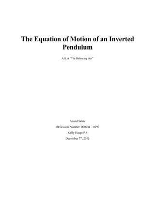
11. PROCESSED DATA: GRAPH 1
ANALYSIS
Again, for the first two seconds of the simulation, there are no external forces applied to the
inverted pendulum, the cart is at position zero, and the angle of the pendulum is at pi relative to the
vertical. At two seconds, a force of 1000N is applied for .01 seconds. The initial force causes the cart to
move to the right, but the controller quickly counter-acts the force by rapidly jerking to the left then
gradually moving to the left to keep the pendulum stable. Meanwhile, the inverted pendulum slightly
tilts left then right, but keeps upright.
In addition, at six seconds, there is another force of -1000N applied for .01 seconds (to the left).
The cart moves to the left, and the controller reacts by quickly moving to the right and keeping still. The
inverted pendulum slightly tilts right then left, but keeps upright.
Force of 1000N
applied for 0.01s
(to the right)
Force of -1000N
applied for 0.01s
(to the left)
The controller reacts
by moving the cart
back-and-forth rapidly
The small scale shows how little the inverted
pendulum is affected, demonstrating the accuracy
of the controller based off the equation of motion

12. PROCESSED DATA: GRAPH 2
ANALYSIS
The same closed-loop scenario occurs as in the previous graph; this graph simply displays the
forces involved. The disturbance force is the same as in the previous graphs. The controller forces occur
immediately after or slightly during the time the disturbance forces are applied, and they counteract the
force with an initial kickback and a relatively gradual stabilization from the kickback. At two seconds,
the controller rapidly moves left, then right, and keeps a small, consistent force. At six seconds, the
The net force includes the
controller and disturbance
forces combined
The controller force
opposes the direction of
the disturbance forces

13. controller quickly moves right, then left, and continues to make minute forces to keep the inverted
pendulum stable.
UNCERTAINTIES
Although this experiment took place in a simulator, there are uncertainties in the linearized
model itself. The simulator is complex, and therefore, isn’t perfect. However, the miniscule inaccuracies
in this experiment are negligible; this is presented in the accuracy of the data in the tables.
4. CONCLUSION AND EVALUATION
CONCLUSION
Ultimately, the control algorithm functioned properly by stabilizing the inverted pendulum after
multiple impacts. The behavior of the cart depended on the algorithm, and the behavior of the algorithm
depended on the state-space model, which was the equation of motion of inverted pendulum. Therefore,
since the eventual functionality was successful, the underlying principles must be true; the equation of
motion of an inverted pendulum is justified.
COMPARISON TO CONTEXT
The state-space model used in this experiment has been accepted for over 50 years. The
procedures from this experiment are derived from control tutorials taught by University of Michigan,
Carnegie Mellon University, and University of Detroit Mercy in conjunction. Because this experiment
was conducted as a simulation, the difference between my results and that of another similar experiment
are little to none.
STRENGTHS AND WEAKNESSES
A definite strength of my experiment is that it was simulated using one of the most popular
applications today: Matlab. It is a justified means of analyzing the validity of control algorithms. On the
other hand, I am not able to visualize the cart unless I had an API for animations. Also, since it was
simulated, I did not encounter inconsistencies in measurement that would have occurred if I had built a
real pendulum balancer. Encoders, both linear and rotational, have their own inconsistencies that may
impact the algorithm. Surprisingly, factors such as mass of the pendulum, mass of the cart, friction
between the pendulum and the cart, and friction between the cart and the rail/ ground do not invalidate
the experiment. The algorithm, since it only takes the angle of the pendulum as an input, is able to adapt
to such changing conditions. Thus, the only weaknesses in building a real pendulum balancer lie in the
inaccuracies of the sensors.
IMPROVEMENTS
I am currently implementing a real pendulum balancer (see Appendix B) to visualize this concept
in action. Moreover, I could implement different, more adaptive control algorithms, each with their own
way of kicking-back and stabilizing, to understand the multifarious forms of such algorithms.

14. 5. WORKS CITED
Works Cited
Messner, Bill, Prof., and Dawn Tilbury, Prof. "Inverted Pendulum: System Modeling." Control
Tutorials for Matlab & Simulink. Matlab, n.d. Web. 7 Dec. 2015.
<http://ctms.engin.umich.edu/CTMS/index.php?example=InvertedPendulum&section=SystemM
odeling>.
Peacock, Finn. An Idiot's Guide to the PID Algorithm. N.p.: n.p., 2008. Print.
"PID Theory Explained." National Instruments. National Instruments, 29 Mar. 2011. Web. 7 Dec. 2015.
<http://www.ni.com/white-paper/3782/en/#top>.
Sekar, Arul Selvan. Personal interview. 21 Aug. 1988.
"Simulink Overview." MathWorks. MathWorks, n.d. Web. 7 Dec. 2015.
<http://www.mathworks.com/products/simulink/>.
"What Are State-Space Models?" MathWorks. MathWorks, 2015. Web. 7 Dec. 2015.
<http://www.mathworks.com/help/ident/ug/what-are-state-space-models.html>.
6. APPENDICES
APPENDIX A – FULL DATA TABLES
OPEN LOOP MODEL
Time
(sec)
Net
Force
(N)
Position
(m)
Angle
(radians)
0.000
0
0
3.141593
0.200
0
-­‐3.9E-­‐19
3.141593
0.400
0
-­‐1.5E-­‐18
3.141593
0.600
0
-­‐3.5E-­‐18
3.141593
0.800
0
-­‐6.1E-­‐18
3.141593
1.000
0
-­‐9.4E-­‐18
3.141593
1.200
0
-­‐1.3E-­‐17
3.141593

15. 1.400
0
-­‐1.8E-­‐17
3.141593
1.600
0
-­‐2.3E-­‐17
3.141593
1.800
0
-­‐2.9E-­‐17
3.141593
2.000
1000
-­‐3.6E-­‐17
3.141593
2.001
0
0.000726
3.14173
2.006
0
0.007983
3.143099
2.031
0
0.04419
3.149933
2.156
0
0.223291
3.184039
2.356
0
0.503421
3.240368
2.556
0
0.77613
3.302631
2.756
0
1.041981
3.375536
2.956
0
1.301533
3.464519
3.156
0
1.555301
3.57605
3.356
0
1.803648
3.717916
3.556
0
2.046547
3.899345
3.756
0
2.283103
4.130795
3.956
0
2.510836
4.42302
4.156
0
2.72505
4.784974
4.356
0
2.91949
5.220054
4.556
0
3.090112
5.720577
4.756
0
3.241407
6.262384
4.956
0
3.387802
6.806573
5.156
0
3.543877
7.313372
5.356
0
3.714118
7.756768
5.556
0
3.893938
8.127338
5.756
0
4.076313
8.4273
5.956
0
4.255956
8.664989
6.156
0
4.430075
8.850938
6.356
0
4.597668
8.995583
6.556
0
4.758689
9.108189
6.756
0
4.913505
9.196537
6.956
0
5.062617
9.267003
7.156
0
5.206531
9.324808
7.356
0
5.345717
9.374295
7.556
0
5.480608
9.419213
7.756
0
5.611604
9.462978
7.956
0
5.739088
9.508919
8.156
0
5.863441
9.56052
8.356
0
5.985053
9.621673
8.556
0
6.104331
9.696943
8.756
0
6.221675
9.791848
8.956
0
6.337424
9.913141
9.156
0
6.451697
10.06902

16. 9.356
0
6.564062
10.26914
9.556
0
6.672953
10.52412
9.756
0
6.774903
10.84417
9.956
0
6.864242
11.23637
10
0
6.881552
11.33249
CLOSED LOOP MODEL
time
(sec)
Net
force
(N)
Position
(m)
Angle
(radians)
Disturbance
Force
(N)
Controller
Force
(N)
0
0
0
3.141593
0
0
0.2
0
-­‐3.9E-­‐19
3.141593
0
0
0.4
0
-­‐1.5E-­‐18
3.141593
0
0
0.6
0
-­‐3.5E-­‐18
3.141593
0
0
0.8
0
-­‐6.1E-­‐18
3.141593
0
0
1
0
-­‐9.4E-­‐18
3.141593
0
0
1.2
0
-­‐1.3E-­‐17
3.141593
0
0
1.4
0
-­‐1.8E-­‐17
3.141593
0
0
1.6
0
-­‐2.3E-­‐17
3.141593
0
0
1.8
0
-­‐2.9E-­‐17
3.141593
0
0
2
1000
-­‐3.6E-­‐17
3.141593
1000
0
2.001000
-­‐0.27874
0.000726
3.14173
0
-­‐0.27874
2.003374
-­‐1.44442
0.00417
3.142379
0
-­‐1.44442
2.007779
-­‐3.01463
0.010518
3.143577
0
-­‐3.01463
2.014174
-­‐4.37555
0.019571
3.145286
0
-­‐4.37555
2.022669
-­‐5.24443
0.031179
3.147476
0
-­‐5.24443
2.033631
-­‐5.63616
0.045326
3.150148
0
-­‐5.63616
2.047759
-­‐5.68874
0.062079
3.153314
0
-­‐5.68874
2.066296
-­‐5.52751
0.081523
3.156997
0
-­‐5.52751
2.091493
-­‐5.19893
0.103479
3.161175
0
-­‐5.19893
2.12733
-­‐4.65726
0.12642
3.165594
0
-­‐4.65726
2.176086
-­‐3.83725
0.143759
3.169083
0
-­‐3.83725
2.207408
-­‐3.32731
0.147646
3.170019
0
-­‐3.32731
2.238731
-­‐2.81962
0.146772
3.170108
0
-­‐2.81962
2.277092
-­‐2.21216
0.140313
3.169272
0
-­‐2.21216
2.319422
-­‐1.57282
0.12778
3.167416
0
-­‐1.57282
2.356675
-­‐1.07255
0.1133
3.165203
0
-­‐1.07255
2.386845
-­‐0.75597
0.099916
3.163143
0
-­‐0.75597
2.415882
-­‐0.47342
0.086116
3.161022
0
-­‐0.47342
2.450591
-­‐0.16707
0.068955
3.158399
0
-­‐0.16707
2.492228
0.146588
0.048116
3.155255
0
0.146588
2.533096
0.405866
0.028078
3.15229
0
0.405866
2.566229
0.524563
0.012505
3.150037
0
0.524563
2.594662
0.582981
-­‐0.0002
3.148243
0
0.582981

17. 2.625863
0.642311
-­‐0.0133
3.146443
0
0.642311
2.664572
0.692539
-­‐0.02823
3.144473
0
0.692539
2.707376
0.731789
-­‐0.04292
3.142646
0
0.731789
2.744599
0.731328
-­‐0.05413
3.141355
0
0.731328
2.774385
0.666937
-­‐0.0621
3.140512
0
0.666937
2.803134
0.614412
-­‐0.06897
3.139851
0
0.614412
2.837934
0.560239
-­‐0.07627
3.139237
0
0.560239
2.879991
0.502172
-­‐0.08377
3.13874
0
0.502172
2.921081
0.464141
-­‐0.08986
3.138478
0
0.464141
2.953999
0.383526
-­‐0.09401
3.138401
0
0.383526
2.982114
0.303382
-­‐0.0971
3.138413
0
0.303382
3.013218
0.242765
-­‐0.10012
3.138497
0
0.242765
3.052142
0.185077
-­‐0.10343
3.138685
0
0.185077
3.095266
0.153444
-­‐0.10662
3.138972
0
0.153444
3.124815
0.089101
-­‐0.10862
3.139198
0
0.089101
3.154364
0.045492
-­‐0.11052
3.13944
0
0.045492
3.191609
0.012089
-­‐0.11283
3.139755
0
0.012089
3.235125
0.003659
-­‐0.11551
3.140122
0
0.003659
3.26573
-­‐0.03348
-­‐0.11743
3.14037
0
-­‐0.03348
3.296335
-­‐0.05648
-­‐0.11941
3.140604
0
-­‐0.05648
3.333712
-­‐0.066
-­‐0.12193
3.140869
0
-­‐0.066
3.376045
-­‐0.05167
-­‐0.12495
3.141135
0
-­‐0.05167
3.414348
-­‐0.03121
-­‐0.12786
3.141341
0
-­‐0.03121
3.445213
-­‐0.0616
-­‐0.13034
3.141482
0
-­‐0.0616
3.473945
-­‐0.07838
-­‐0.13274
3.141595
0
-­‐0.07838
3.507649
-­‐0.07693
-­‐0.13568
3.141704
0
-­‐0.07693
3.548618
-­‐0.05936
-­‐0.13941
3.141807
0
-­‐0.05936
3.590189
-­‐0.01685
-­‐0.14337
3.141881
0
-­‐0.01685
3.624379
-­‐0.01789
-­‐0.14674
3.141919
0
-­‐0.01789
3.653034
-­‐0.04265
-­‐0.14964
3.141938
0
-­‐0.04265
3.683454
-­‐0.0447
-­‐0.15278
3.141947
0
-­‐0.0447
3.721122
-­‐0.03343
-­‐0.15674
3.141946
0
-­‐0.03343
3.763956
8.44E-­‐05
-­‐0.16132
3.141931
0
8.44E-­‐05
3.794462
-­‐0.01415
-­‐0.16463
3.141912
0
-­‐0.01415
3.824967
-­‐0.01797
-­‐0.16796
3.141889
0
-­‐0.01797
3.862203
-­‐0.0095
-­‐0.17206
3.141857
0
-­‐0.0095
3.904527
0.018337
-­‐0.17672
3.141819
0
0.018337
3.94298
0.047046
-­‐0.18097
3.141783
0
0.047046
3.97395
0.019829
-­‐0.1844
3.141753
0
0.019829
4.002644
0.003032
-­‐0.18758
3.141727
0
0.003032
4.036205
0.002597
-­‐0.19128
3.141698
0
0.002597
4.077071
0.015207
-­‐0.19577
3.141667
0
0.015207
4.118736
0.050928
-­‐0.20032
3.141639
0
0.050928

18. 4.153082
0.044672
-­‐0.20406
3.141619
0
0.044672
4.181776
0.013557
-­‐0.20718
3.141603
0
0.013557
4.212089
0.004659
-­‐0.21046
3.14159
0
0.004659
4.249605
0.007566
-­‐0.2145
3.141577
0
0.007566
4.292432
0.031564
-­‐0.21909
3.141566
0
0.031564
4.323047
0.012022
-­‐0.22236
3.14156
0
0.012022
4.353663
0.002729
-­‐0.22563
3.141555
0
0.002729
4.390899
0.005015
-­‐0.22958
3.141552
0
0.005015
4.433086
0.026369
-­‐0.23405
3.141552
0
0.026369
4.471437
0.049314
-­‐0.23809
3.141553
0
0.049314
4.50245
0.01973
-­‐0.24137
3.141554
0
0.01973
4.531258
0.000873
-­‐0.24441
3.141555
0
0.000873
4.564891
-­‐0.00183
-­‐0.24795
3.141558
0
-­‐0.00183
4.605704
0.0087
-­‐0.25224
3.141562
0
0.0087
4.647235
0.042242
-­‐0.2566
3.141568
0
0.042242
4.68154
0.035052
-­‐0.26021
3.141571
0
0.035052
4.710305
0.004409
-­‐0.26324
3.141573
0
0.004409
4.740719
-­‐0.00435
-­‐0.26644
3.141576
0
-­‐0.00435
4.77827
-­‐0.00111
-­‐0.27039
3.14158
0
-­‐0.00111
4.821002
0.02337
-­‐0.27488
3.141584
0
0.02337
4.851621
0.004362
-­‐0.2781
3.141586
0
0.004362
4.88224
-­‐0.0043
-­‐0.28133
3.141588
0
-­‐0.0043
4.919457
-­‐0.00118
-­‐0.28525
3.14159
0
-­‐0.00118
4.961621
0.021072
-­‐0.28969
3.141593
0
0.021072
4.999978
0.044897
-­‐0.29373
3.141595
0
0.044897
5.031011
0.016211
-­‐0.29701
3.141595
0
0.016211
5.059832
-­‐0.00201
-­‐0.30006
3.141595
0
-­‐0.00201
5.093456
-­‐0.00404
-­‐0.30361
3.141595
0
-­‐0.00404
5.134247
0.007192
-­‐0.30791
3.141596
0
0.007192
5.17577
0.041258
-­‐0.31229
3.141597
0
0.041258
5.21009
0.034673
-­‐0.31592
3.141597
0
0.034673
5.238872
0.004416
-­‐0.31897
3.141596
0
0.004416
5.269287
-­‐0.00407
-­‐0.32218
3.141595
0
-­‐0.00407
5.306822
-­‐0.00057
-­‐0.32615
3.141595
0
-­‐0.00057
5.349538
0.024058
-­‐0.33066
3.141595
0
0.024058
5.380174
0.005259
-­‐0.33391
3.141594
0
0.005259
5.410809
-­‐0.00331
-­‐0.33715
3.141593
0
-­‐0.00331
5.448022
-­‐0.00015
-­‐0.34108
3.141593
0
-­‐0.00015
5.490163
0.022043
-­‐0.34553
3.141593
0
0.022043
5.528506
0.045677
-­‐0.34958
3.141594
0
0.045677
5.559549
0.017083
-­‐0.35287
3.141593
0
0.017083
5.588388
-­‐0.00114
-­‐0.35592
3.141592
0
-­‐0.00114
5.622021
-­‐0.00324
-­‐0.35947
3.141591
0
-­‐0.00324

19. 5.662801
0.007883
-­‐0.36378
3.141592
0
0.007883
5.704303
0.041708
-­‐0.36816
3.141592
0
0.041708
5.73862
0.035018
-­‐0.37179
3.141592
0
0.035018
5.767415
0.004802
-­‐0.37484
3.141591
0
0.004802
5.797844
-­‐0.00374
-­‐0.37806
3.141591
0
-­‐0.00374
5.835382
-­‐0.00031
-­‐0.38202
3.141591
0
-­‐0.00031
5.878082
0.024201
-­‐0.38653
3.141591
0
0.024201
5.90872
0.005361
-­‐0.38977
3.141591
0
0.005361
5.939359
-­‐0.00326
-­‐0.39301
3.141591
0
-­‐0.00326
5.976569
-­‐0.00014
-­‐0.39694
3.141591
0
-­‐0.00014
6
-­‐1000.01
-­‐0.39942
3.14159
-­‐1000
-­‐0.00864
6.001
0.269925
-­‐0.40025
3.141453
0
0.269925
6.006
2.449772
-­‐0.40801
3.140088
0
2.449772
6.019289
4.969051
-­‐0.42808
3.136566
0
4.969051
6.033104
5.613006
-­‐0.44758
3.133159
0
5.613006
6.050767
5.658859
-­‐0.47021
3.129235
0
5.658859
6.073106
5.433015
-­‐0.4951
3.124965
0
5.433015
6.10307
5.01853
-­‐0.52222
3.120393
0
5.01853
6.143832
4.374648
-­‐0.54858
3.116104
0
4.374648
6.190121
3.558037
-­‐0.56565
3.113566
0
3.558037
6.217672
3.143418
-­‐0.57026
3.113049
0
3.143418
6.245224
2.706834
-­‐0.57139
3.113149
0
2.706834
6.282635
2.122992
-­‐0.56823
3.114105
0
2.122992
6.328654
1.438029
-­‐0.55858
3.116273
0
1.438029
6.358431
1.081189
-­‐0.54983
3.118096
0
1.081189
6.388208
0.748117
-­‐0.53971
3.120138
0
0.748117
6.426055
0.366202
-­‐0.52557
3.122925
0
0.366202
6.469864
-­‐0.02106
-­‐0.50836
3.126247
0
-­‐0.02106
6.499957
-­‐0.19814
-­‐0.49651
3.128502
0
-­‐0.19814
6.530049
-­‐0.35127
-­‐0.48495
3.13068
0
-­‐0.35127
6.567472
-­‐0.50859
-­‐0.4713
3.133228
0
-­‐0.50859
6.610487
-­‐0.65206
-­‐0.45695
3.135876
0
-­‐0.65206
6.641112
-­‐0.68431
-­‐0.44778
3.137552
0
-­‐0.68431
6.671736
-­‐0.70276
-­‐0.43956
3.139043
0
-­‐0.70276
6.709012
-­‐0.71133
-­‐0.43087
3.140601
0
-­‐0.71133
6.751227
-­‐0.71047
-­‐0.42279
3.142031
0
-­‐0.71047
6.789554
-­‐0.69233
-­‐0.41701
3.143037
0
-­‐0.69233
6.820527
-­‐0.61882
-­‐0.41335
3.143663
0
-­‐0.61882
6.849324
-­‐0.55347
-­‐0.4107
3.144106
0
-­‐0.55347
6.882985
-­‐0.49166
-­‐0.40844
3.14447
0
-­‐0.49166
6.923841
-­‐0.42716
-­‐0.40677
3.144717
0
-­‐0.42716
6.965371
-­‐0.38445
-­‐0.4061
3.144785
0
-­‐0.38445
6.999636
-­‐0.31604
-­‐0.40617
3.14473
0
-­‐0.31604

20. 7.028373
-­‐0.23695
-­‐0.40659
3.144623
0
-­‐0.23695
7.058799
-­‐0.18033
-­‐0.40732
3.144459
0
-­‐0.18033
7.09639
-­‐0.12993
-­‐0.40854
3.144204
0
-­‐0.12993
7.139146
-­‐0.10163
-­‐0.41021
3.143869
0
-­‐0.10163
7.169729
-­‐0.05001
-­‐0.41151
3.143614
0
-­‐0.05001
7.200312
-­‐0.01349
-­‐0.41285
3.143354
0
-­‐0.01349
7.237532
0.01125
-­‐0.41449
3.143042
0
0.01125
7.279746
0.012942
-­‐0.41628
3.142704
0
0.012942
7.318134
0.004351
-­‐0.41781
3.14242
0
0.004351
7.349149
0.041999
-­‐0.41893
3.142213
0
0.041999
7.37793
0.065615
-­‐0.41988
3.142039
0
0.065615
7.411534
0.070856
-­‐0.42088
3.141858
0
0.070856
7.452346
0.059886
-­‐0.42191
3.141672
0
0.059886
7.493914
0.022579
-­‐0.42277
3.14152
0
0.022579
7.528244
0.024795
-­‐0.42333
3.141422
0
0.024795
7.556999
0.050723
-­‐0.42369
3.141359
0
0.050723
7.587381
0.053748
-­‐0.424
3.141308
0
0.053748
7.624909
0.042841
-­‐0.42427
3.141265
0
0.042841
7.667659
0.009348
-­‐0.42444
3.141239
0
0.009348
7.69829
0.021857
-­‐0.42449
3.141235
0
0.021857
7.72892
0.024305
-­‐0.42448
3.141239
0
0.024305
7.76614
0.014091
-­‐0.42442
3.141254
0
0.014091
7.808294
-­‐0.01542
-­‐0.4243
3.141281
0
-­‐0.01542
7.846638
-­‐0.04494
-­‐0.42415
3.141311
0
-­‐0.04494
7.877673
-­‐0.02042
-­‐0.424
3.14134
0
-­‐0.02042
7.906504
-­‐0.00557
-­‐0.42386
3.141367
0
-­‐0.00557
7.940138
-­‐0.00685
-­‐0.42369
3.141399
0
-­‐0.00685
7.980926
-­‐0.02128
-­‐0.42349
3.141437
0
-­‐0.02128
8.022436
-­‐0.05768
-­‐0.4233
3.141472
0
-­‐0.05768
8.056748
-­‐0.05243
-­‐0.42314
3.141501
0
-­‐0.05243
8.085535
-­‐0.02305
-­‐0.42302
3.141523
0
-­‐0.02305
8.115961
-­‐0.01512
-­‐0.4229
3.141544
0
-­‐0.01512
8.153503
-­‐0.01891
-­‐0.42278
3.141566
0
-­‐0.01891
8.196212
-­‐0.04341
-­‐0.42266
3.141586
0
-­‐0.04341
8.226845
-­‐0.02428
-­‐0.42259
3.141599
0
-­‐0.02428
8.257477
-­‐0.01525
-­‐0.42253
3.141609
0
-­‐0.01525
8.294689
-­‐0.01771
-­‐0.42247
3.141619
0
-­‐0.01771
8.336832
-­‐0.03898
-­‐0.42243
3.141625
0
-­‐0.03898
8.375178
-­‐0.06174
-­‐0.4224
3.141629
0
-­‐0.06174
8.406222
-­‐0.0324
-­‐0.42238
3.141631
0
-­‐0.0324
8.435059
-­‐0.0135
-­‐0.42237
3.141632
0
-­‐0.0135
8.468689
-­‐0.01063
-­‐0.42237
3.141632
0
-­‐0.01063
8.509468
-­‐0.0209
-­‐0.42238
3.141629
0
-­‐0.0209

21. 8.550974
-­‐0.05395
-­‐0.42239
3.141625
0
-­‐0.05395
8.585293
-­‐0.0467
-­‐0.42241
3.141622
0
-­‐0.0467
8.614086
-­‐0.01605
-­‐0.42241
3.14162
0
-­‐0.01605
8.644514
-­‐0.00711
-­‐0.42243
3.141617
0
-­‐0.00711
8.682049
-­‐0.01014
-­‐0.42244
3.141613
0
-­‐0.01014
8.72475
-­‐0.03429
-­‐0.42247
3.141608
0
-­‐0.03429
8.75539
-­‐0.01526
-­‐0.42248
3.141606
0
-­‐0.01526
8.78603
-­‐0.0065
-­‐0.42249
3.141603
0
-­‐0.0065
8.82324
-­‐0.00949
-­‐0.42251
3.1416
0
-­‐0.00949
8.865373
-­‐0.03154
-­‐0.42252
3.141596
0
-­‐0.03154
8.903713
-­‐0.05509
-­‐0.42254
3.141593
0
-­‐0.05509
8.934761
-­‐0.02655
-­‐0.42254
3.141592
0
-­‐0.02655
8.963606
-­‐0.00837
-­‐0.42254
3.141592
0
-­‐0.00837
8.99724
-­‐0.00631
-­‐0.42255
3.14159
0
-­‐0.00631
9.038014
-­‐0.01752
-­‐0.42255
3.141589
0
-­‐0.01752
9.079511
-­‐0.0514
-­‐0.42256
3.141587
0
-­‐0.0514
9.113828
-­‐0.04481
-­‐0.42256
3.141587
0
-­‐0.04481
9.142628
-­‐0.01472
-­‐0.42255
3.141588
0
-­‐0.01472
9.173061
-­‐0.00627
-­‐0.42255
3.141588
0
-­‐0.00627
9.210597
-­‐0.0098
-­‐0.42255
3.141588
0
-­‐0.0098
9.253292
-­‐0.0344
-­‐0.42255
3.141587
0
-­‐0.0344
9.283933
-­‐0.01565
-­‐0.42254
3.141588
0
-­‐0.01565
9.314574
-­‐0.0071
-­‐0.42254
3.141589
0
-­‐0.0071
9.351783
-­‐0.01029
-­‐0.42253
3.141589
0
-­‐0.01029
9.393912
-­‐0.03246
-­‐0.42253
3.141589
0
-­‐0.03246
9.432252
-­‐0.05606
-­‐0.42253
3.141589
0
-­‐0.05606
9.463302
-­‐0.02757
-­‐0.42252
3.14159
0
-­‐0.02757
9.492149
-­‐0.00938
-­‐0.42251
3.141591
0
-­‐0.00938
9.525783
-­‐0.00729
-­‐0.42251
3.141591
0
-­‐0.00729
9.566555
-­‐0.01842
-­‐0.42251
3.141591
0
-­‐0.01842
9.60805
-­‐0.05219
-­‐0.42251
3.141591
0
-­‐0.05219
9.642368
-­‐0.04553
-­‐0.4225
3.141591
0
-­‐0.04553
9.67117
-­‐0.01537
-­‐0.42249
3.141592
0
-­‐0.01537
9.701604
-­‐0.00684
-­‐0.42249
3.141593
0
-­‐0.00684
9.73914
-­‐0.01027
-­‐0.42249
3.141593
0
-­‐0.01027
9.781832
-­‐0.03475
-­‐0.42249
3.141592
0
-­‐0.03475
9.812474
-­‐0.01594
-­‐0.42248
3.141593
0
-­‐0.01594
9.843116
-­‐0.00732
-­‐0.42248
3.141593
0
-­‐0.00732
9.880325
-­‐0.01044
-­‐0.42247
3.141593
0
-­‐0.01044
9.922452
-­‐0.03253
-­‐0.42248
3.141592
0
-­‐0.03253
9.960791
-­‐0.05607
-­‐0.42248
3.141591
0
-­‐0.05607
9.991842
-­‐0.02755
-­‐0.42247
3.141592
0
-­‐0.02755
10
-­‐0.01279
-­‐0.42247
3.141593
0
-­‐0.01279

22. APPENDIX B – PHYSICAL INVERTED PENDULUM ROBOT
The development of this robot is going relatively quickly. My goal is to finish it within one month. The
picture above is of the prototype. The robot is very well designed, with a low center of gravity. With the
right materials and measurements, it should have low friction and low error. The entire chassis,
pendulum mounts, and several other parts are completely laser cut, so human error in construction is
little to none. Once I’m finished, I hope to aggregate the documentation into a research report and post
the designs and instructions online.