Robust control theory based performance investigation of an inverted pendulum system using simulink
•
0 likes•44 views

Mustefa
![Vol-6 Issue-2 2020 IJARIIE-ISSN(O)-2395-4396
11638 www.ijariie.com 809
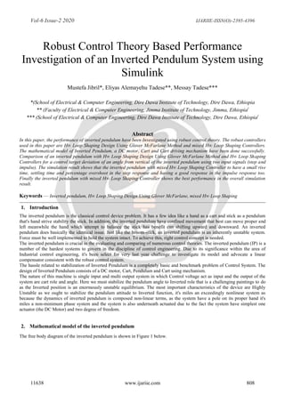
Figure 1: Free body diagrams of the inverted pendulum system.
Summing the forces in the free body diagram of the cart in the horizontal direction, you get the following equation of motion:
1Mz Dz Q F
The force exerted in the horizontal direction due to the moment on the pendulum is determined as follows:
2
r F I
I
F
r
mI
I
mI
Component of this force in the direction of Q is cosmI
The component of the centripetal force acting along the horizontal axis is as follows:
2
2 2
2
I
F
r
mI
I
mI
Component of this force in the direction of Q is
2
sinmI
Summing the forces in the Free Body Diagram of the pendulum in the horizontal direction, you can get an equation for Q:
2
cos sin 2Q mz mI mI
If you substitute this equation [2] into the first equation [1], you get the first equation of motion for this system:
2
cos sin 3M m z Dz mI mI F To get the second equation of motion, sum the forces
perpendicular to the pendulum. This axis is chosen to simplify mathematical complexity. Solving the system along this axis
ends up saving you a lot of algebra. Just as the previous equation is obtained, the vertical components of those forces are
considered here to get the following equation:
sin cos sin cos 4W Q mg mI mz
To get rid of the P and N terms in the equation above, sum the moments around the centroid of the pendulum to get the
following equation:
sin cos 5WI QI I
Combining these last two equations, you get the second dynamic equation:
2
sin cos 6I mI mgI mIz
The set of equations completely defining the dynamics of the inverted pendulum are:
2
cos sinM m z Dz mI mI F ](data:image/gif;base64,R0lGODlhAQABAIAAAAAAAP///yH5BAEAAAAALAAAAAABAAEAAAIBRAA7)
Recommended
Recommended
More Related Content
What's hot
What's hot (20)
Similar to Robust control theory based performance investigation of an inverted pendulum system using simulink
Similar to Robust control theory based performance investigation of an inverted pendulum system using simulink (20)
More from Mustefa Jibril
More from Mustefa Jibril (20)
Recently uploaded
Recently uploaded (20)
Robust control theory based performance investigation of an inverted pendulum system using simulink
- 1. Vol-6 Issue-2 2020 IJARIIE-ISSN(O)-2395-4396 11638 www.ijariie.com 808 Robust Control Theory Based Performance Investigation of an Inverted Pendulum System using Simulink Mustefa Jibril*, Eliyas Alemayehu Tadese**, Messay Tadese*** *(School of Electrical & Computer Engineering, Dire Dawa Institute of Technology, Dire Dawa, Ethiopia ** (Faculty of Electrical & Computer Engineering, Jimma Institute of Technology, Jimma, Ethiopia) *** (School of Electrical & Computer Engineering, Dire Dawa Institute of Technology, Dire Dawa, Ethiopia) Abstract In this paper, the performance of inverted pendulum have been Investigated using robust control theory. The robust controllers used in this paper are H∞ Loop Shaping Design Using Glover McFarlane Method and mixed H∞ Loop Shaping Controllers. The mathematical model of Inverted Pendulum, a DC motor, Cart and Cart driving mechanism have been done successfully. Comparison of an inverted pendulum with H∞ Loop Shaping Design Using Glover McFarlane Method and H∞ Loop Shaping Controllers for a control target deviation of an angle from vertical of the inverted pendulum using two input signals (step and impulse). The simulation result shows that the inverted pendulum with mixed H∞ Loop Shaping Controller to have a small rise time, settling time and percentage overshoot in the step response and having a good response in the impulse response too. Finally the inverted pendulum with mixed H∞ Loop Shaping Controller shows the best performance in the overall simulation result. Keywords — Inverted pendulum, H∞ Loop Shaping Design Using Glover McFarlane, mixed H∞ Loop Shaping 1. Introduction The inverted pendulum is the classical control device problem. It has a few idea like a hand as a cart and stick as a pendulum that's hand strive stability the stick. In addition, the inverted pendulum have confined movement that best can move proper and left meanwhile the hand which attempt to balance the stick has benefit can shifting upward and downward. An inverted pendulum does basically the identical issue. Just like the broom-stick, an inverted pendulum is an inherently unstable system. Force must be well implemented to hold the system intact. To achieve this, right control concept is needed. The inverted pendulum is crucial in the evaluating and comparing of numerous control theories. The inverted pendulum (IP) is a number of the hardest systems to govern in the discipline of control engineering. Due to its significance within the area of Industrial control engineering, it's been select for very last year challenge to investigate its model and advocate a linear compensator consistent with the robust control system. The hassle related to stabilization of Inverted Pendulum is a completely basic and benchmark problem of Control System. The design of Inverted Pendulum consists of a DC motor, Cart, Pendulum and Cart using mechanism. The nature of this machine is single input and multi output system in which Control voltage act as input and the output of the system are cart role and angle. Here we must stabilize the pendulum angle to Inverted role that is a challenging paintings to do as the Inverted position is an enormously unstable equilibrium. The most important characteristics of the device are Highly Unstable as we ought to stabilize the pendulum attitude to Inverted function, it's miles an exceedingly nonlinear system as because the dynamics of inverted pendulum is composed non-linear terms, as the system have a pole on its proper hand it's miles a non-minimum phase system and the system is also underneath actuated due to the fact the system have simplest one actuator (the DC Motor) and two degree of freedom. 2. Mathematical model of the inverted pendulum The free body diagram of the inverted pendulum is shown in Figure 1 below.
- 2. Vol-6 Issue-2 2020 IJARIIE-ISSN(O)-2395-4396 11638 www.ijariie.com 809 Figure 1: Free body diagrams of the inverted pendulum system. Summing the forces in the free body diagram of the cart in the horizontal direction, you get the following equation of motion: 1Mz Dz Q F The force exerted in the horizontal direction due to the moment on the pendulum is determined as follows: 2 r F I I F r mI I mI Component of this force in the direction of Q is cosmI The component of the centripetal force acting along the horizontal axis is as follows: 2 2 2 2 I F r mI I mI Component of this force in the direction of Q is 2 sinmI Summing the forces in the Free Body Diagram of the pendulum in the horizontal direction, you can get an equation for Q: 2 cos sin 2Q mz mI mI If you substitute this equation [2] into the first equation [1], you get the first equation of motion for this system: 2 cos sin 3M m z Dz mI mI F To get the second equation of motion, sum the forces perpendicular to the pendulum. This axis is chosen to simplify mathematical complexity. Solving the system along this axis ends up saving you a lot of algebra. Just as the previous equation is obtained, the vertical components of those forces are considered here to get the following equation: sin cos sin cos 4W Q mg mI mz To get rid of the P and N terms in the equation above, sum the moments around the centroid of the pendulum to get the following equation: sin cos 5WI QI I Combining these last two equations, you get the second dynamic equation: 2 sin cos 6I mI mgI mIz The set of equations completely defining the dynamics of the inverted pendulum are: 2 cos sinM m z Dz mI mI F
- 3. Vol-6 Issue-2 2020 IJARIIE-ISSN(O)-2395-4396 11638 www.ijariie.com 810 2 sin cosI mI mgI mIz These two equations are non-linear and need to be linearized for the operating range. Since the pendulum is being stabilized at an unstable equilibrium position, which is ‘Pi’ radians from the stable equilibrium position, this set of equations should be linearized about theta = Pi. Assume that theta = Pi + ø, (where ø represents a small angle from the vertical upward direction). Therefore, cos (theta) = -1, sin (theta) = -ø, and (d (theta)/dt) ^2 = 0. After linearization the two equations of motion become (where u represents the input): 7M m z Dz mI u 2 8I mI mgI mIz The transfer function of Inverted Pendulum, a DC motor, Cart and Cart driving system will be 3 2 1.3 0.272 0.34 0.8 1 s s E s s s s Where E (s) = Error Voltage, and s = Angular Position of the Pendulum. The parameters of the system is shown in Table 1 below Table 1 Parameters of the inverted pendulum Model parameter symbols Symbols value Mass of the Cart M 1 kg Mass of the Pendulum m 0.3 kg Friction of the Cart D 0.000 N/m/sec Length of pendulum to Center of Gravity L 0.26m Moment of Inertia (Pendulum) I 0.007 kg-m2 Radius of Pulley, r 0.04 m Force applied to the cart F Cart Position Coordinate z Pendulum Angle with the vertical 3. The Proposed Controllers Design 3.1 H∞ Mixed-Sensitivity Synthesis Method for Robust Control Loop Shaping Design of Inverted Pendulum Mixed sensitivity (MS) control is a routine named as such due to the transfer function shaping methods used. The MS control routine aims to find a controller that gives the desired closed-loop sensitivity transfer functions S, R, and T which is given by 1 S I GK 1 R K I GK 1 T GK I GK Figure 2 shows the relevant inverted pendulum system control architecture with H∞ mixed sensitivity controller Figure 2 The inverted pendulum with H∞ mixed sensitivity controller
- 4. Vol-6 Issue-2 2020 IJARIIE-ISSN(O)-2395-4396 11638 www.ijariie.com 811 The S and T are called the sensitivity and complementary sensitivity, respectively. R measures the control effort. The returned controller K is such that S, R, and T satisfy the following loop-shaping inequalities: 1 1 1 2 1 3 ( ( )) ( ( )) ( ( )) ( ( )) ( ( )) ( ( )) S j W j R j W j T j W j Where γ = GAM. Thus, the inverses of W 1 and W 3 determine the shapes of sensitivity S and complementary sensitivity T. Typically, you choose a W 1 that is large inside the desired control bandwidth to achieve good disturbance attenuation (i.e., performance). Similarly, you typically choose a W 3 that is large outside the control bandwidth, which helps to ensure good stability margin. Here in this system we choose the three weighting functions W1, W2 and W3 as 2 1 2 2 2 2 3 4 3 2 4 6 3 50 5 7 3 10 20 7.6 6 4 3 2 s s W s s s s W s s W s s s s 3.2 H∞ Loop Shaping Design Using Glover McFarlane Method Control of Inverted Pendulum The multivariable systems is difficult not only because multi-input and multi-output (MIMO) are involved but also due to the failure of phase information in MIMO argument that makes it impossible to predict the steadfastness of the closed-loop system formed by the unity feedback. However, based on the robust stabilization against perturbations on normalized coprime factorizations, a formatting method, known as the H ∞ loop-shaping design using Glover-McFarlane method has been developed. The H ∞ loop-shaping design agency augments the plant with appropriately chosen weights so that the frequency feedback of the open-loop system (the weighted plant) is reshaped in order to meet the closed-loop attainment requirements. Then a robust controller is synthesized to meet the stability. The block diagram of the inverted pendulum system with H ∞ Loop shaping design using Glover McFarlane controller is shown in Figure 3 bellow. Figure 3 Block diagram of the inverted pendulum system with H ∞ Loop shaping design using Glover McFarlane controller We choose a pre compensator, W1 and a post compensator, W2 transfer functions as 2 1 3 2 3 2 2 4 3 2 2 3 2 4 2 2 2 3 s s W s s s s s s W s s s s 4. Result and Discussion Here in this section, the comparison of the inverted pendulum with H∞ mixed sensitivity and H ∞ Loop shaping design using Glover McFarlane controllers using the error voltage input step and impulse have been done. 4.1 Simulation of the inverted pendulum without Controller The Simulink model and the angle from the vertical output for a step and impulse error voltage input is shown in Figure 4, Figure 5 and Figure 6 respectively.
- 5. Vol-6 Issue-2 2020 IJARIIE-ISSN(O)-2395-4396 11638 www.ijariie.com 812 Figure 4 Simulink model of inverted pendulum without controller Figure 5 Step response of inverted pendulum without controller Figure 6 Impulse response of inverted pendulum without controller 4.2 Simulation of the inverted pendulum with H∞ mixed sensitivity and H ∞ Loop shaping design using Glover McFarlane controllers using step input error voltage signal The Simulink model of the inverted pendulum with H∞ mixed sensitivity and H ∞ Loop shaping design using Glover McFarlane controllers using step input error voltage signal is shown in Figure 7 below. Figure 7 Simulink model of the proposed controllers for step input signal The simulation output of the angle from the vertical for a step error voltage input signal of the inverted pendulum with H∞ mixed sensitivity and H ∞ Loop shaping design using Glover McFarlane controllers is shown in Figure 8 below.
- 6. Vol-6 Issue-2 2020 IJARIIE-ISSN(O)-2395-4396 11638 www.ijariie.com 813 Figure 8 Step response 4.3 Simulation of the inverted pendulum with H∞ mixed sensitivity and H ∞ Loop shaping design using Glover McFarlane controllers using Impulse input error voltage signal The Simulink model of the inverted pendulum with H∞ mixed sensitivity and H ∞ Loop shaping design using Glover McFarlane controllers using impulse input error voltage signal is shown in Figure 9 below. Figure 9 Simulink model of the proposed controllers for impulse input signal The simulation output of the angle from the vertical for an impulse error voltage input signal of the inverted pendulum with H∞ mixed sensitivity and H ∞ Loop shaping design using Glover McFarlane controllers is shown in Figure 10 below. Figure 10 Impulse response 4.4 Numerical Values of the Simulation Output The numerical values of the rise time, settling time and percentage overshoot of the proposed controllers are shown in Table 2 below Table 2 Proposed controller’s performance numerical result No Controller Rise Time s % Overshoot Settling Time s 1 H∞ mixed sensitivity 0.0667 14.4 % 1.8 2 H ∞ Loop shaping 0.27 32.7 % 4.8
- 7. Vol-6 Issue-2 2020 IJARIIE-ISSN(O)-2395-4396 11638 www.ijariie.com 814 5. Conclusion In this paper, performance investigation of an inverted pendulum system using robust control theory have been analyzed and simulated successfully. The mathematical model of Inverted Pendulum, a DC motor, Cart and Cart driving mechanism have been developed. The inverted pendulum with H∞ mixed sensitivity and H ∞ Loop shaping design using Glover McFarlane controllers have been designed and the comparison of the inverted pendulum with H∞ mixed sensitivity and H ∞ Loop shaping design using Glover McFarlane controllers using step and impulse input error voltage signals have been done using Matlab/Simulink. The simulation results prove that the inverted pendulum with H∞ mixed sensitivity controller shows improvement in minimizing the rise time, settling time and percentage overshoot than the inverted pendulum with H ∞ Loop shaping design using Glover McFarlane controller. Finally the comparative and simulation results prove the effectiveness of the inverted pendulum with H∞ mixed sensitivity controller. REFERENCES [1]. Saqib I et al. “Advanced Sliding Mode Control Techniques for Inverted Pendulum: Modelling and Simulation” Engineering Science and Technology, an International Journal, Vol. 21, Issue 4 pp. 753-759, 2018. [2]. Xiaojie Su et al. “Event Triggered Fuzzy Control of Nonlinear Systems with its Application to Inverted Pendulum Systems” Automatica, Vol. 94, pp. 236-248, 2018. [3]. H Gritli et al. “Robust Feedback Control of the under actuated Inertia Wheel Inverted Pendulum under Parametric Uncertainties and Subject to External Disturbances: LMI Formulation” Journal of the Franklin Institute, Vol. 355, Issue 18, 2018. [4]. Q Xu et al. “Balancing a Wheeled Inverted Pendulum with a Single Accelerometer in the Presence of Time Delay” Journal of Vibration and Control, 2017. [5]. I Yigit et al. “Model Free Sliding Mode Stabilization Control of a Real Rotary Inverted Pendulum” Journal of Vibration and Control, 2017. [6]. J Wen et al. “Stabilizing a Rotary Inverted Pendulum Base on Logarithmic Lyapunov Function” Journal of Control Science and Engineering, 2017. [7]. Wei Chen et al. “Simulation of a Triple Inverted Pendulum Based on Fuzzy Control” World Journal of Engineering and Technology, Vol. 4, No. 2, 6 pages, 2016. [8]. Mukhtar F et al. “Genetic Algorithm and Particle Swarm Optimization Based Cascade Interval Type 2 Fuzzy PD Controller for Rotary Inverted Pendulum System” Journal of Mathematical Problems in Engineering, Vol. 2015, 15 pages, 2015. [9]. LB Prasad et al. “Optimal Control of Nonlinear Inverted Pendulum System using PID Controller and LQR: Performance Analysis without and with Disturbance Input” International Journal of Automation and Control, 2014. [10]. M Yue et al. “Dynamic Balance and Motion Control for Wheeled Inverted Pendulum Vehicle via hierarchical Sliding Mode Approach” Journal of Systems and Control, 2014. [11]. Liang Zhang et al. “Fuzzy Modelling and Control for a Class of Inverted Pendulum System” Journal of Advanced Stochastic Control Systems with Engineering Applications, 6 pages, 2014.