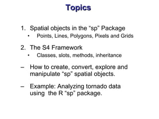
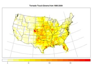
This document summarizes the use of spatial data analysis in R using the sp package. It discusses how to create and manipulate spatial point, line, polygon and grid objects. It provides an example of analyzing Colorado tornado data and counting storms in hexagonal grids over the United States to demonstrate spatial analysis techniques in R.


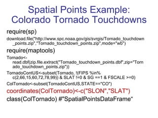
![str(ColTornado) Formal class 'SpatialPointsDataFrame' [package "sp"] with 5 slots ..@ data :'data.frame': 1762 obs. of 25 variables: ..@ coords.nrs : int [1:2] 16 15 ; data columns ..@ coords : num [1:1762, 1:2] -103 -102 -102 -102 -104 ... ;coordinates longitude, lattitude .. ..- attr(*, "dimnames")=List of 2 ;column names ..@ bbox : num [1:2, 1:2] -109 37 -102 41 .. ..- attr(*, "dimnames")=List of 2 ..@ proj4string:Formal class 'CRS' [package "sp"] with 1 slots ;projection string (we will assign one later)](https://image.slidesharecdn.com/sp-12940180559908-phpapp02/85/R-Spatial-Analysis-using-SP-8-320.jpg)

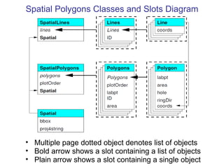
![#Create grid lines and grid text along with plot layouts latlonlines<-gridlines(ColMapSpLines,easts= -110:-101 ) latlonlinesLayout<-list("sp.lines",latlonlines,lty=2,col="pink") latlontext<-gridat(latlonlines) #Split for better use of positioning latlontextE<-latlontext[latlontext$pos==1,] latlontextN<-latlontext[latlontext$pos==2,] latlontextLayoutE<-list("sp.text",coordinates(latlontextE), parse(text=as.character(latlontextE$labels)),offset=latlontextE$offset[1]/2,pos=1,col="brown") latlontextLayoutN<-list("sp.text",coordinates(latlontextN), parse(text=as.character(latlontextN$labels)),offset=latlontextN$offset[1]/2,pos=2,col="green")](https://image.slidesharecdn.com/sp-12940180559908-phpapp02/85/R-Spatial-Analysis-using-SP-13-320.jpg)
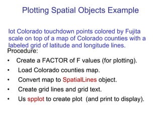
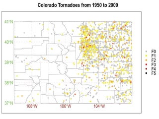
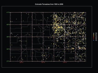
![spLayout<-list(ColMapSpLinesLayout, latlonlinesLayout, latlontextLayoutE, latlontextLayoutN) spplot(ColTornado["FSCALE_FACTOR"], pch=20, alpha=.8, key.space="right”, xlim=c(-109.8,101.5), ylim=c(36.5,41.5), col.regions= c("grey","yellow","orange","red","brown", "black"), main="Colorado Tornadoes from 1950 to 2009", sp.layout=spLayout) The spplot function plots one color for each FSCAL_FACTOR level. uses trellis graphics from lattice package. adds layers in sp.layout in order. uses alpha for transparency. (density plot)](https://image.slidesharecdn.com/sp-12940180559908-phpapp02/85/R-Spatial-Analysis-using-SP-14-320.jpg)
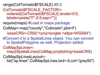
![require(rgdal) #rgdal code in green projInfo()[55,] # lcc Lambert Conformal Conic lambertCRS<- " +proj=lcc +lat_1=60 +lat_2=30 +lon_0=-100" #Spacing (and lack of) intentional in CRS string. #project() uses matrix with longitude latitude cols. #CRS string cannot contain reference ellipsoid. res=project( cbind(Tornado2$SLON,Tornado2$SLAT ), lambertCRS) Tornado2$x=res[,1]; Tornado2$y=res[,2] #Make copy, convert to SpatialPointsDataFrame US_sp=Tornado2 coordinates(US_sp)=~x+y](https://image.slidesharecdn.com/sp-12940180559908-phpapp02/85/R-Spatial-Analysis-using-SP-19-320.jpg)
![#overlay locations, returns hexagon location locations=overlay(US_sp,HexPols) #Use of table function to count points in hexagon counttable<-as.data.frame ( table( factor(locations, levels=1: length(HexPols@polygons) ) ) , row.names= sapply(HexPols@polygons, function(x) [email_address] ) ) [,"Freq",drop=F] colnames(counttable)<-"counts“ HexPolsDf = SpatialPolygonsDataFrame( HexPols, counttable, match.ID = TRUE)](https://image.slidesharecdn.com/sp-12940180559908-phpapp02/85/R-Spatial-Analysis-using-SP-22-320.jpg)
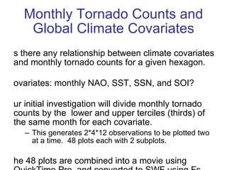
![Monthly Covariate Procedure Download covariates and unstack by month and year. Generate monthly quantiles (terciles) for the covariates. Merge covariates with climate data. Create SpatialPointsDataFrame (SPDF) from merged dataset. Overlay SPDF onto hexagon SpatialPolygons tiling. Add hexagon id as “hex” column to SPDF. Split SPDF by Hexagon id and remove empty hexagons from hexagon tiling (i.e. id not in SPDF@data[“hex”]) For each covariate and each month, table the tornado touchdown points in the given month by the terciles of the given covariate observed in that month. Create SpatialPolygonsDataFrame from result. Plot each figure as PNG and combine into movie.](https://image.slidesharecdn.com/sp-12940180559908-phpapp02/85/R-Spatial-Analysis-using-SP-27-320.jpg)
![#Download Covariates and create Quantiles #Climate Covariates from 1861-2009 source("data/climateCovariates.R") # Green colored functions from: source("funs/tsupport.R") startend<-1950:2009 #tornado years covariates<- make.cov.unstacked (climateCovariates, se=startend,cov=c("soi","nao","sst","sun")) monthlyquantiles<- as.array.list ( lapply( split(covariates[,-(1:2)], covariates$Month), function(x) out<- apply(x,2,quantile,probs=c(1/4,1/3,1/2,2/3,3/4) ) ) , name="Month" )](https://image.slidesharecdn.com/sp-12940180559908-phpapp02/85/R-Spatial-Analysis-using-SP-28-320.jpg)
![TornadoClimate<-merge(TornadoContUS, covariates, by.x=c("YEAR","MONTH"), by.y=c("Year","Month")) projcords=project( as.matrix(TornadoClimate[c("SLON","SLAT")]), lambertCRS) #As before TC<-TornadoClimate TC$x<-projcords[,1];TC$y<-projcords[,2] coordinates(TC)=~x+y hexagonNumber<-overlay(TC,HexPols) TC$Hex<-hexagonNumber](https://image.slidesharecdn.com/sp-12940180559908-phpapp02/85/R-Spatial-Analysis-using-SP-29-320.jpg)
![#Split Hexagons (Will order by hex number) TCsplit <-split(TC@data,TC$Hex) names( TCsplit )<-sapply(HexPols@polygons, function(x) x@ID)[as.numeric(names( TCsplit ))] #Remove empty tiles from hexagon tiling. (V10.1 R) HexPolsMissing<-HexPols[names(TCsplit),] #Create Yearly Frequency yearspersplit <- count.storms (x=covariates,cut=3,col.name="Month", quantiles = monthlyquantiles,Year%in%startend) splitcounts<-data.frame(t(sapply( TCsplit , function(x) count.storms ( x,cut=3, FSCALE>=1 & YEAR %in% startend , quantiles = monthlyquantiles ) ) / yearspersplit ) ) #Create SpatialPolygonsDataFrame splitcountsSPDF<-SpatialPolygonsDataFrame(HexPolsMissing,splitcounts)](https://image.slidesharecdn.com/sp-12940180559908-phpapp02/85/R-Spatial-Analysis-using-SP-30-320.jpg)
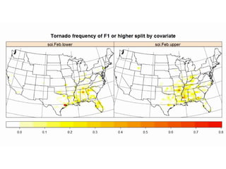
![#Create Images dir.create("./monthlyclimatepng") png(file="./monthlyclimatepng/plot%03d.png", width=1080, height=600, bg="white",res=120) for(i in 1:48) #4 covariates 12 months { #Plot lower and upper thirds in each plot print( spplot(splitcountsSPDF[, c(3*i-2,3*i) ], lty=0, col.regions=rev(heat.colors(100))[1:90], sp.layout=list(l1,G1), as.table=T , main="Tornado frequency of F1 or higher split by covariate", colorkey=list(space="bottom")) ) } dev.off()](https://image.slidesharecdn.com/sp-12940180559908-phpapp02/85/R-Spatial-Analysis-using-SP-31-320.jpg)


![Spatial_Data_Analysis_with_open_source_softwares[1]](https://cdn.slidesharecdn.com/ss_thumbnails/8db4d971-8e8c-4fd8-8682-b20e5d6cd65f-161221072847-thumbnail.jpg?width=640&height=640&fit=bounds)