Downloaded 30 times


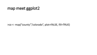

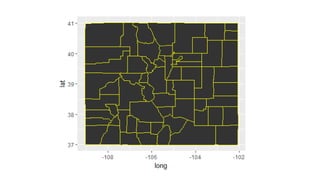
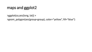
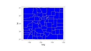
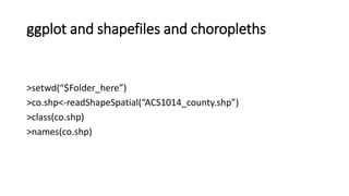

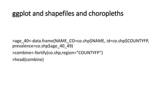
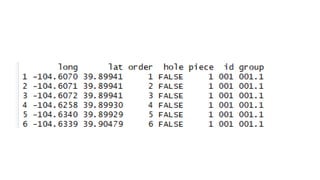
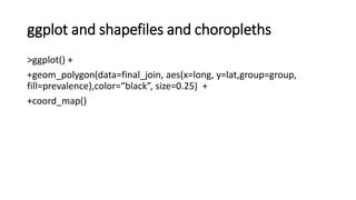
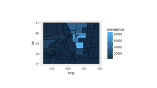
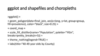
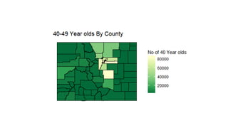
![ggplot and shapefiles and choropleths
>merge.shp<-merge(combine, age_40, by=“id”, all.x=TRUE)
>final_join<-merge.shp[order(merge.shp$order),]](https://image.slidesharecdn.com/rspatialpresentation-171116195103/85/R-spatial-presentation-48-320.jpg)
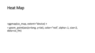
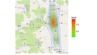


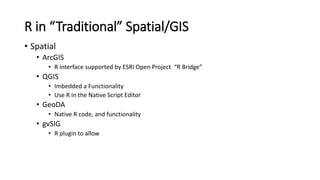
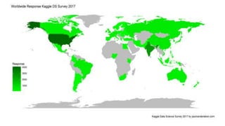
This document discusses using R for spatial and geospatial analysis. It provides an overview of key R packages for working with spatial data like ggplot2, rgdal, and maptools. It also demonstrates how to create basic maps from shapefiles, perform spatial joins to add data attributes, and generate choropleth and heat maps for visualization and analysis. The document serves as a tutorial for getting started with spatial analysis and visualization using open-source R tools and libraries.


![Spatial_Data_Analysis_with_open_source_softwares[1]](https://cdn.slidesharecdn.com/ss_thumbnails/8db4d971-8e8c-4fd8-8682-b20e5d6cd65f-161221072847-thumbnail.jpg?width=640&height=640&fit=bounds)


