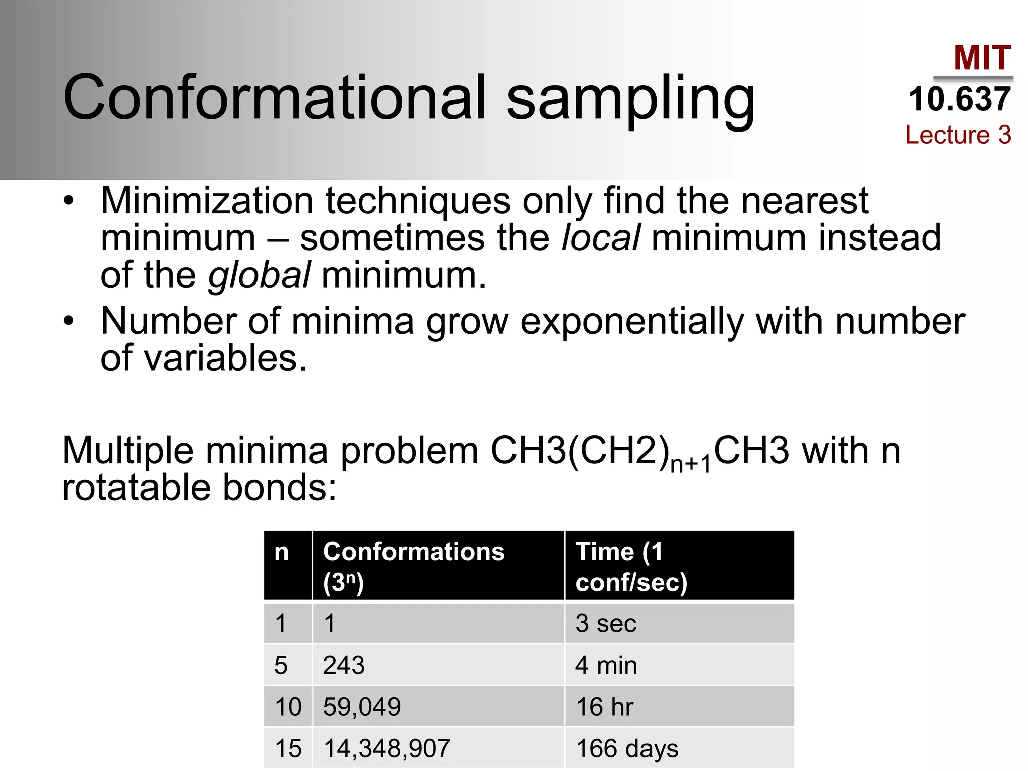
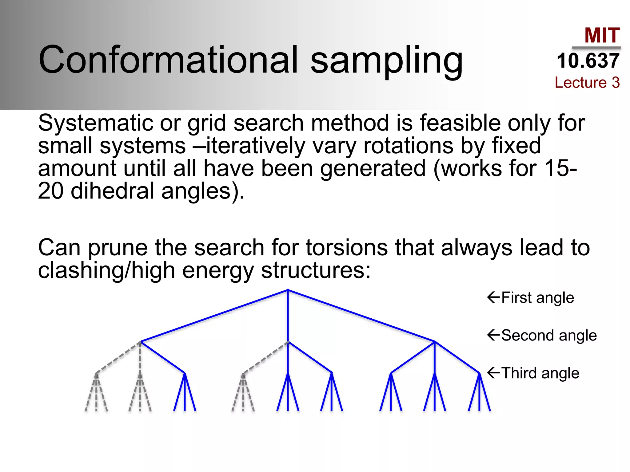
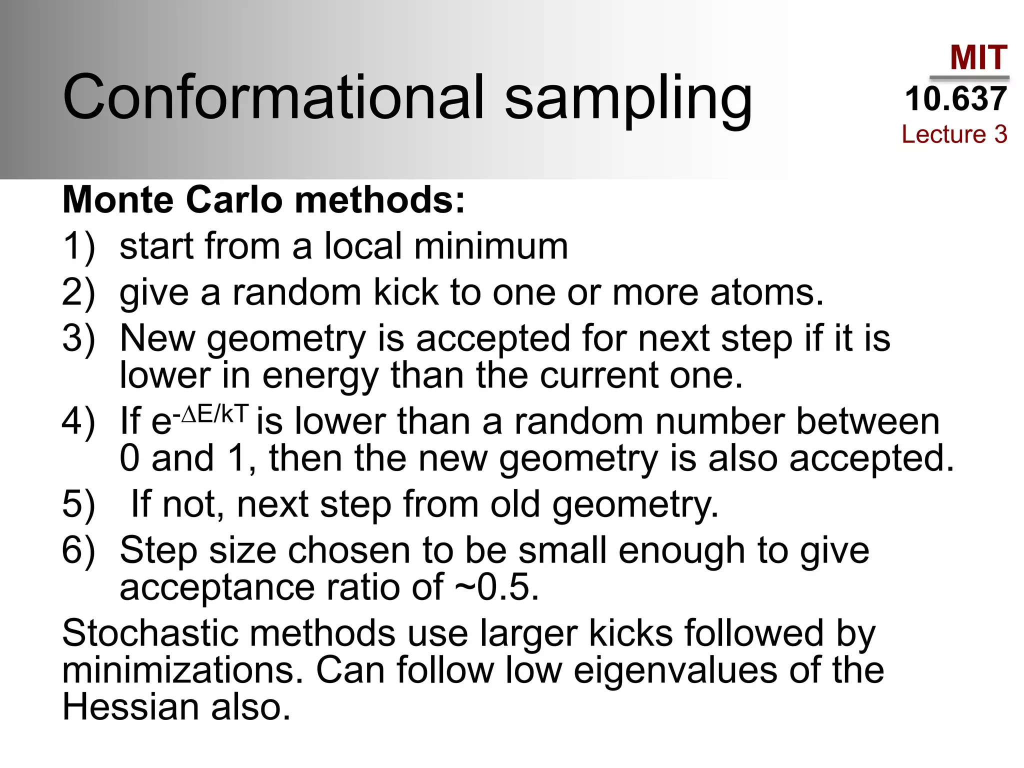
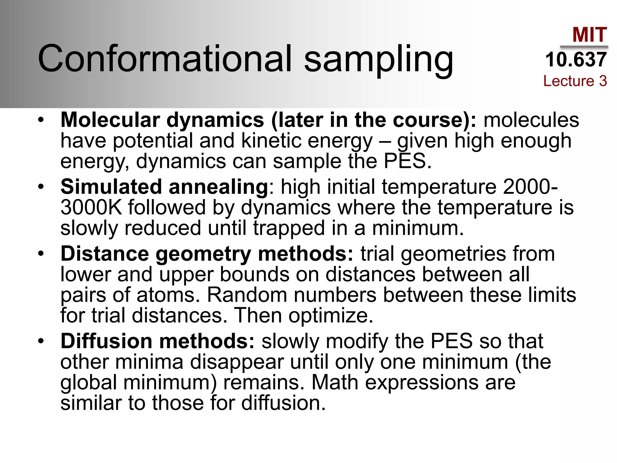
The document outlines the principles of potential energy surfaces (PES) in molecular geometry optimizations, discussing the Born-Oppenheimer approximation, the separation of variables, and various methods for PES mapping. It covers optimization techniques such as steepest descent, conjugate gradient, and Newton-Raphson methods, including their advantages, challenges, and improvements. Additionally, it addresses conformational sampling methods like Monte Carlo, molecular dynamics, and genetic algorithms, highlighting their applications in exploring the energy landscape of molecular systems.

1. Geometry optimizations and
potential energy surfaces
Heather J Kulik
09-11-14

2. MIT
10.637
Lecture 3
Where do potential energy
surfaces come from?
• Force field discussion implicitly assumed there
was some potential energy function describing
bonding in a molecule.
• Comes from quantum mechanical descriptions: we
have light electrons that move quickly and heavy,
slow moving nuclei.
• Can separate the variables and contributions so
that nuclei and electrons are not coupled
(exceptions are e.g. light elements like hydrogen
atom tunneling).

3. MIT
10.637
Lecture 3
The Born Oppenheimer
Approximation
• From the electronic point of view, the
nuclei are stationary.
• Electronic wavefunction depeneds
parametrically on nuclear coordinates (i.e.
depends only on position of nuclei, not on
momentum).
• BO approx only introduces error of 10-4 au
for light molecule H2. Small contribution
compared to other errors.

4. MIT
10.637
Lecture 3
Separation of variables
nuc
KE
el
KE
el-nuc
attraction
el-el
repulsion
nuc-nuc
repulsion:
parametric
The overall Hamiltonian (Htot) is applied to a wavefunction dependent on
nuclear coordinates (R) and electronic coordinates (r).
Can separate electronic and nuclear quantities:
Electronic energy depends parameterically on R due to fixed potential from
nuclei:

5. MIT
10.637
Lecture 3
Molecular degrees of freedom
Linear Nonlinear
Translational 3 3
Rotational 2 3
Vibrational 3N-5 3N-6
For zero field,
potential energy
derived only from
vibrational
coordinates.
e.g. H2O: N = 3, 3 normal modes
symmetric stretch asymmetric stretchbend
Degrees of freedom in a potential energy surface:
This gets large very quickly !

6. MIT
10.637
Lecture 3
Molecular degrees of freedom
• Another way to think of it is in terms of
internal degrees of freedom.
• A single atom has no degrees of freedom,
just an origin.
• Second atom is defined by distance from the
first – 1 degree of freedom.
• Third atom must be specified by two
distances or one distance and one angle – 3
degrees of freedom. (3N-6)
• Each additional atom requires 3 more
degrees of freedom.

7. MIT
10.637
Lecture 3
Mapping a complete PES
For very small
systems: we can
map out a fully ab
initio potential
energy surface.
e.g. CH4+Cl, CH5+,
etc. see work of
Bowman group.
But this PES mapping is impractical
for anything but very small systems.

8. MIT
10.637
Lecture 3
Mapping PESs in practice
• Complete PESs for polyatomic molecules are very
hard to visualize.
• Usually we take slices through the PES that
involve 1-2 coordinates.
• Usually we aim to get the minimum energy for all
other coordinates with fixed values of the varied
coordinates along the potential energy surface.

9. MIT
10.637
Lecture 3
Energy minimizations
Ñf =
¶f
¶x1
, ,
¶f
¶xn
æ
è
ç
ö
ø
÷
Ñf = 0
Force = -Ñ(Energy)Minimize:
Gradient on our PES in
terms of all coordinates
(internal, cartesian):
For :
Any stationary point
(a) local minimum,
(b) global minimum,
(c) saddle point.
What we usually
want!
Coordinates can be cartesian or internal coordinates (distances/angles/dihedrals) –
or transform between two.

10. MIT
10.637
Lecture 3
The Hessian/Force matrix
(3N-6)x(3N-6) matrix
with elements:
Hij ( f ) =
¶2
f
¶xi¶xj
H( f ) =
¶2
f
¶x1
2
¶2
f
¶x1¶x2
¶2
f
¶x1¶xn
¶2
f
¶x2¶x1
¶2
f
¶x2
2
¶2
f
¶x2¶xn
¶2
f
¶xn¶x1
¶2
f
¶xn¶x2
¶2
f
¶xn
2
é
ë
ê
ê
ê
ê
ê
ê
ê
ê
ê
ê
ù
û
ú
ú
ú
ú
ú
ú
ú
ú
ú
ú
(3N-6)
(3N-6)
Approximate PES around stationary point by harmonic potentials.

11. MIT
10.637
Lecture 3
The Hessian/Force matrix
Diagonalize Hessian
(eigenvalue problem)
From E. Eliav,
Tel Aviv U
minimum maximum saddle point
eklj
(k)
= Hijli
(k)
i=1
n
å
ek = mwk
2
Eigenvalues: Eigenvectors:
normal
coordinates
Harmonic
frequencies
εk>0 εk<0 εk>0, except one εj<0
ωk all real ωk all imaginary one imaginary ωj on RC

12. MIT
10.637
Lecture 3
Optimizations
• Many methods assume an analytic
gradient of the energy is available.
• Some methods assume the Hessian or an
approximation of it is available.
• Can carry out a constrained optimization:
fix a geometrical parameter and optimize
subject t this constraint by rewriting
function as a Lagrange function.

13. MIT
10.637
Lecture 3
Steepest descent
Optimization direction:
Size of step determined by line
search: calculate E at several
points along . Fit a
polynomial to calculated values
and find the minimum to get
point 2.
g = -ÑE
ri+1 = ri +
ligi
gi
Update coordinates:
Reduce λ near minimum.

14. MIT
10.637
Lecture 3
Steepest descent
Pros: Fast when far from minimum,
local minimization guaranteed.
Cons: slow descent for certain
PESs, can oscillate near minimum.
Often used for cases where far from
minimum and then switch to another
method when you get closer to the
minimum.

15. MIT
10.637
Lecture 3
Conjugate gradient
Improvement over SD method.
First step is same as SD:
determined via line search.
Subsequent steps: linear
combination of negative
gradient and preceding search
direction.
Pro: Using history, faster
convergence near minimum.

16. MIT
10.637
Lecture 3
Conjugate gradient
Updated position:
l is from line search.
Gradient directions:
Avoids undoing previous steps.

17. MIT
10.637
Lecture 3
Newton-Raphson method
Expands the true function to second order around the current
point x0:
Set derivative with respect to (x-x0) equal to zero:
gradient Hessian
Hessian Gradient

18. MIT
10.637
Lecture 3
Newton-Raphson method
Transform to a coordinate system
(x’) where the Hessian is diagonal then
the steps are:
Projection of gradient along
Hessian eigenvector
Hessian eigenvalue
Interpretation is that you need a larger step if you have a large gradient or if
the force constant is smaller. Exact if quadratic PES.

19. MIT
10.637
Lecture 3
Newton-Raphson Method
Problems:
1) if a Hessian eigenvalue is negative, step direction will be
along gradient and increase the value, possibly
converging at a saddle point.
2) Inverse Hessian sets step size. If one of the eigenvalues
is close to zero, step size goes to infinity – can take
everything outside of where the second-order expansion
is valid.
Can set a trust-radius to limit step size.
Advantage: Second order convergence near stationary point,
linear convergence further away.

20. MIT
10.637
Lecture 3
Newton-Raphson
improvements
Can adjust step size for cases with negative eigenvalues
with a shift parameter (l):
l can be the lowest Hessian eigevalue so the denominator
is always positive.
Methods that do this are called augmented Hessian, level-
shifted NR, or Eigenvector following.
Rational-Function Optimization:
(solve iteratively)

21. MIT
10.637
Lecture 3
Newton-Raphson
improvements
Actually obtaining the Hessian (a 3N-6x3N-6 matrix) is difficult for most practical
systems.
1) Start with a guess for the Hessian instead, e.g. the unit matrix – this makes it
behave like a steepest descent or a guess based on geometrical properties.
2) In subsequent steps, gradients at previous and current points are used to make
the Hessian better. After two steps, Hessian becomes a good approximation to
the exact Hessian in direction defined by those two points.
--e.g. Broyden-Fletcher-Goldfarb-Shanno (BFGS) method:
BFGS is preferred because it tends to keep Hessian positive-definite.

22. MIT
10.637
Lecture 3
Minimizations… in practice
• Explicit Hessian methods accurate but too expensive
for large molecules (9N2, 27N3). Approximations,
updating.
• In AMBER: SD,CG, BFGS, following low freq modes
for struct. change.
• May use only CG (gradient history ~ implicit treatment
of Hessian)
• Combinatorial explosion: large molecules
(eg.rotatable bonds), many possible conformers. Need
better ways to seek out global minimum: genetic
algorithms, Monte Carlo, etc.

23. MIT
10.637
Lecture 3
Conformational sampling
• Minimization techniques only find the nearest
minimum – sometimes the local minimum instead
of the global minimum.
• Number of minima grow exponentially with number
of variables.
Multiple minima problem CH3(CH2)n+1CH3 with n
rotatable bonds:
n Conformations
(3n)
Time (1
conf/sec)
1 1 3 sec
5 243 4 min
10 59,049 16 hr
15 14,348,907 166 days

24. MIT
10.637
Lecture 3
Conformational sampling
Systematic or grid search method is feasible only for
small systems –iteratively vary rotations by fixed
amount until all have been generated (works for 15-
20 dihedral angles).
Can prune the search for torsions that always lead to
clashing/high energy structures:
First angle
Second angle
Third angle

25. MIT
10.637
Lecture 3
Conformational sampling
Monte Carlo methods:
1) start from a local minimum
2) give a random kick to one or more atoms.
3) New geometry is accepted for next step if it is
lower in energy than the current one.
4) If e-DE/kT is lower than a random number between
0 and 1, then the new geometry is also accepted.
5) If not, next step from old geometry.
6) Step size chosen to be small enough to give
acceptance ratio of ~0.5.
Stochastic methods use larger kicks followed by
minimizations. Can follow low eigenvalues of the
Hessian also.

26. MIT
10.637
Lecture 3
Conformational sampling
• Molecular dynamics (later in the course): molecules
have potential and kinetic energy – given high enough
energy, dynamics can sample the PES.
• Simulated annealing: high initial temperature 2000-
3000K followed by dynamics where the temperature is
slowly reduced until trapped in a minimum.
• Distance geometry methods: trial geometries from
lower and upper bounds on distances between all
pairs of atoms. Random numbers between these limits
for trial distances. Then optimize.
• Diffusion methods: slowly modify the PES so that
other minima disappear until only one minimum (the
global minimum) remains. Math expressions are
similar to those for diffusion.

27. MIT
10.637
Lecture 3
Conformational sampling
Genetic algorithms:
-Example of an evolutionary algorithm.
-Start with a population of structures characterized by
“genes” – e.g. 0s and 1s to represent dihedrals.
-Parent structures generate children having mixture of
parent genes.
-Small probability of mutations in the process.
-Fittest, lowest energy species (10%) are carried to
next generation. Other 90% generated by mating the
40% fittest and allowing for mutations.
-typically proceeds for ~100 generations but
population, mutation, breeding, ratio of children/
parents, local optimizations of the structures, etc can
all be varied.