The document discusses fundamental concepts in quantum mechanics, focusing on the Schrödinger wave equation and its implications for particles in potential wells. It highlights how classical and quantum mechanics differ, emphasizing the non-derivable nature of the Schrödinger equation and the importance of wave functions and their normalization. Additionally, it covers expectations and properties of wave functions, as well as exploring specific scenarios like the infinite square-well potential.
This chapter introduces quantum mechanics, covering key topics such as wave equations, potential wells, and the foundations laid by Richard Feynman.
Mathematical expressions related to quantum mechanics, including functions, derivatives, and wave equations, setting the stage for further discussion.
Discussion on the dual nature of light and matter, questioning the classical derivation of physical phenomena from Maxwell's equations.
Exploration of light waves as probabilistic entities, governed by complex wave equations and properties related to frequency and wavelength.
Brief biographical note on prominent physicists and their influence on modern physics, emphasizing their contributions to biophysics and theoretical physics.
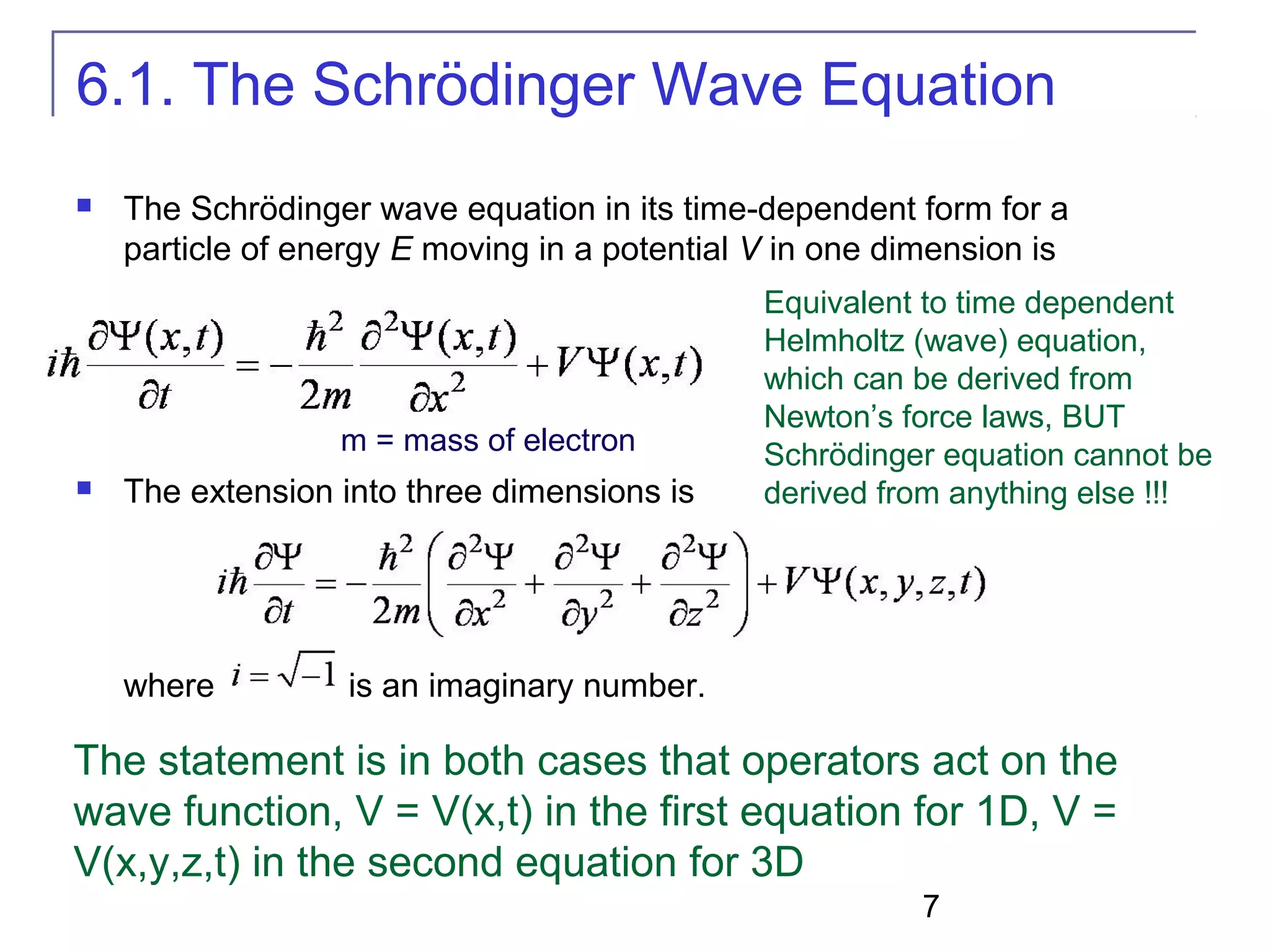
Describes the time-dependent Schrödinger wave equation, key to quantum mechanics, emphasizing its foundational role in physics.
Comparison between Newton’s mechanics and the Schrödinger equation, underlining the superiority of quantum mechanics in fundamental physics.
Analysis of how total energy relates to wave functions, covering concepts like conservation of energy and the importance of complex numbers.
The relationship between constant potential energy and free particle wave functions in quantum mechanics.
Discusses the linearity of Schrödinger's equation, wave function solutions, and the concept of measurement in quantum mechanics.
Describes the characteristics of wave functions for free particles and how they relate to complex numbers and normalization.
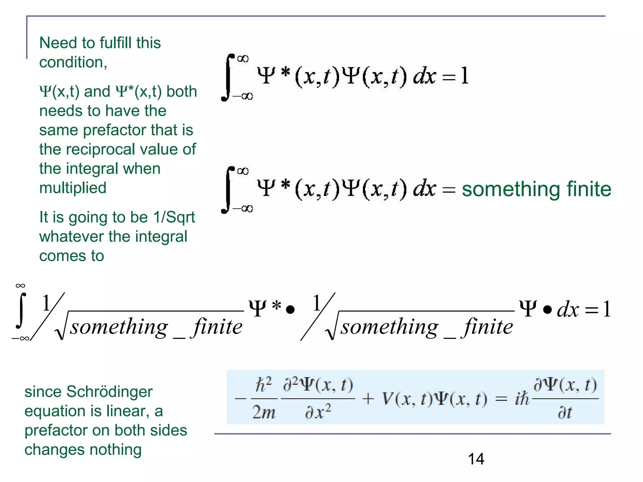
Details on the normalization of wave functions to ensure probability conservation, establishing a fundamental aspect of quantum mechanics.
Further elaboration on normalization of wave functions, ensuring finite probabilities and correct mathematical properties.
Challenges in normalizing wave functions for free particles and the implications of infinite probabilities.
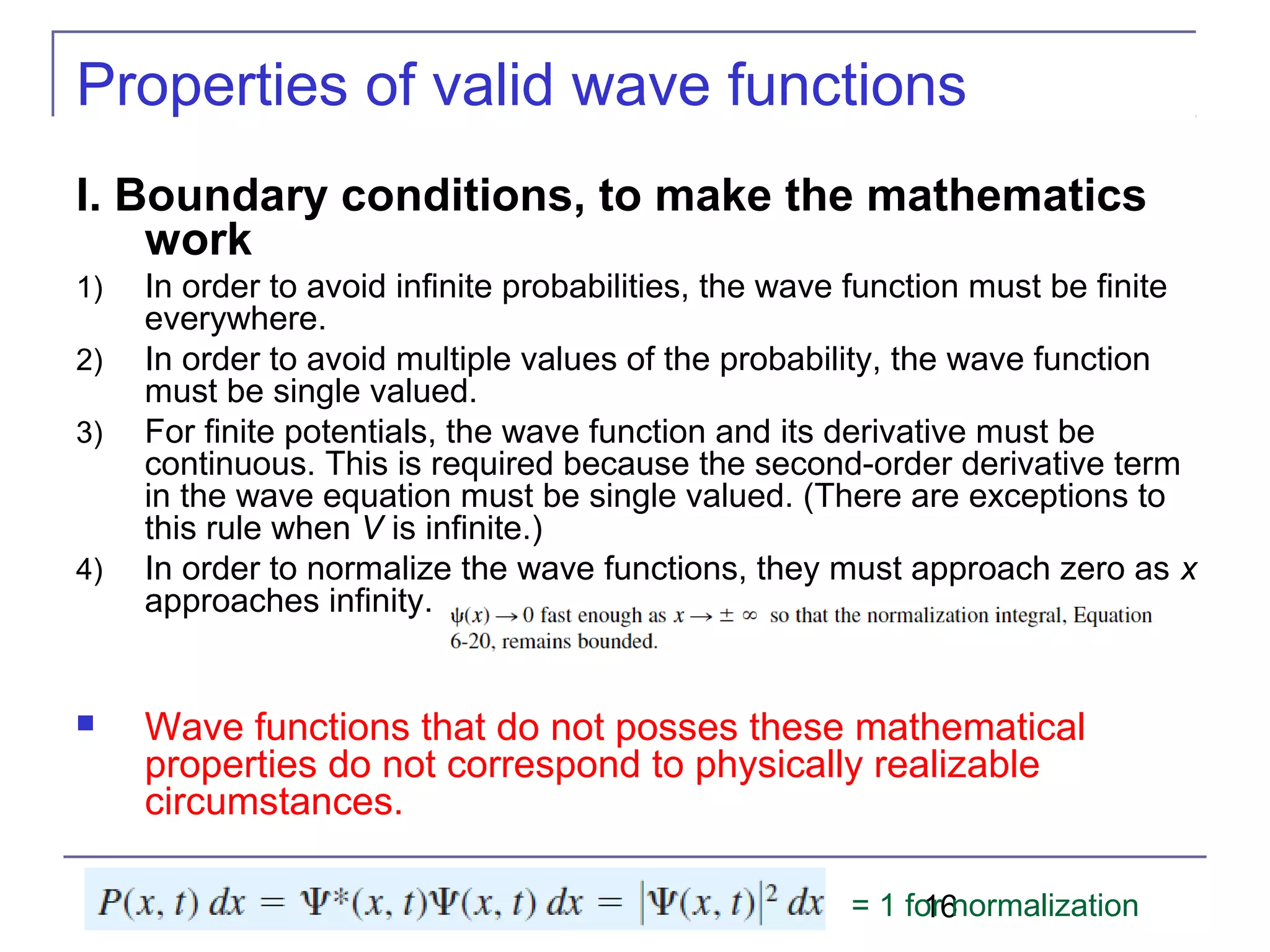
Key properties of valid wave functions, including boundary conditions and requirements for physical realizability.
Further conditions on wave functions to ensure continuity and matching derivatives at boundaries in quantum systems.
Discussion of the time-independent Schrödinger equation and its role in separating variables in quantum systems.
Understanding the form and implications of the time-independent Schrödinger equation in quantum mechanics.
Overview of stationary states and time-independent probability densities in quantum systems.
Introduction to expectation values in quantum mechanics and their significance in measuring physical observables.
Transition from discrete to continuous variables in calculating expectation values using wave functions.
Definitions and implications of the momentum operator in describing quantum mechanical systems.
Details on position and energy operators in quantum mechanics, emphasizing their direct roles in wave functions.
Clarification of how operators are applied to wave functions to extract physical information.
Guidance on creating new operators from classical equations to represent quantum observables.
Discussion on the differences between sharp and fuzzy expectation values in quantum measurements.
Analysis of the implications of eigenvalues on measurement variability in quantum mechanics.
Further details on the significance of eigenvalues in determining discrete energy states in quantum systems.
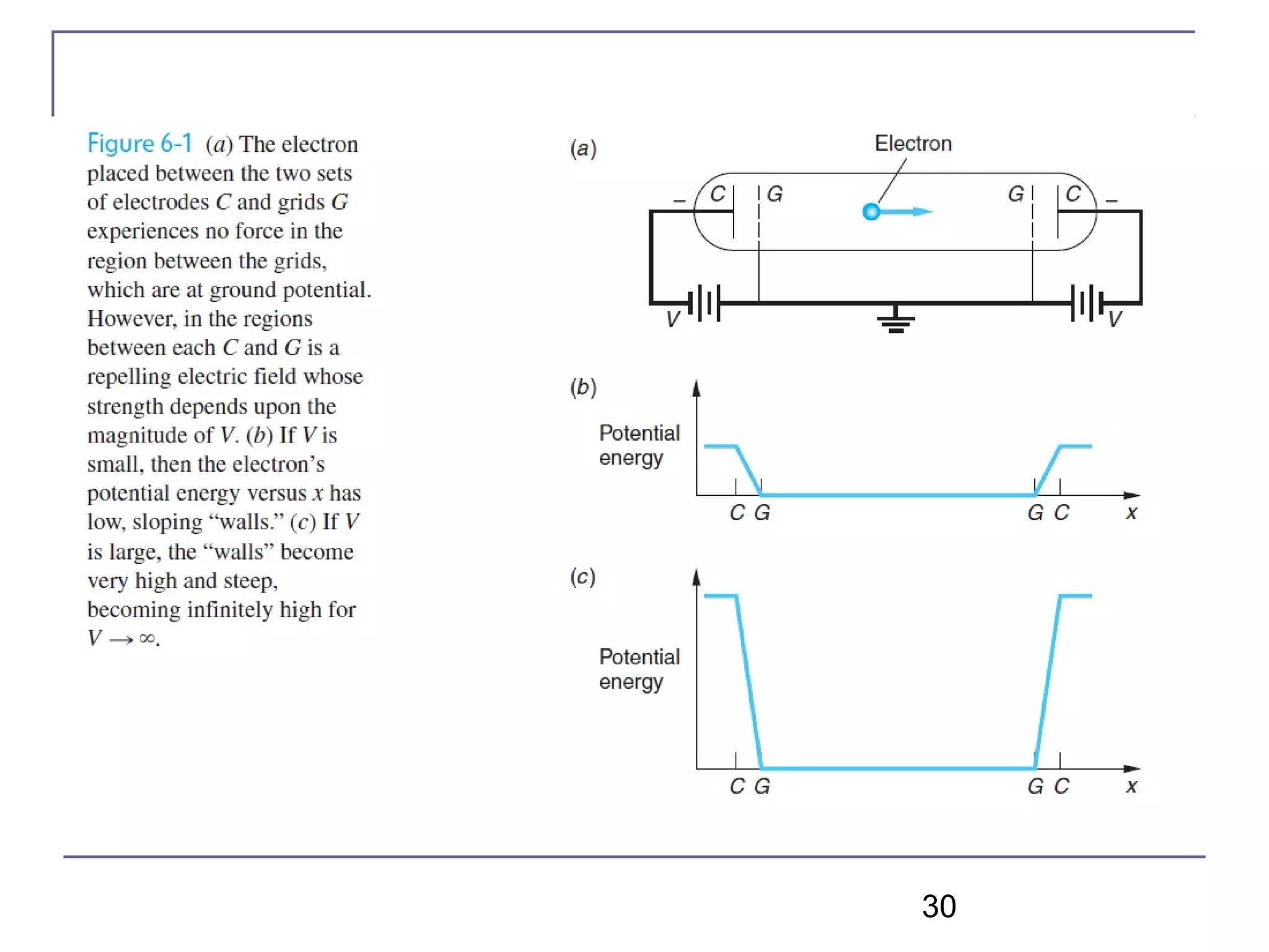
Introduction to the concept of the infinite square well potential and its implications in quantum mechanics.
Details on boundary conditions for the infinite square well, establishing valid wave solutions.
Exploration of quantized energy levels in the infinite square well and their significance in quantum mechanics.
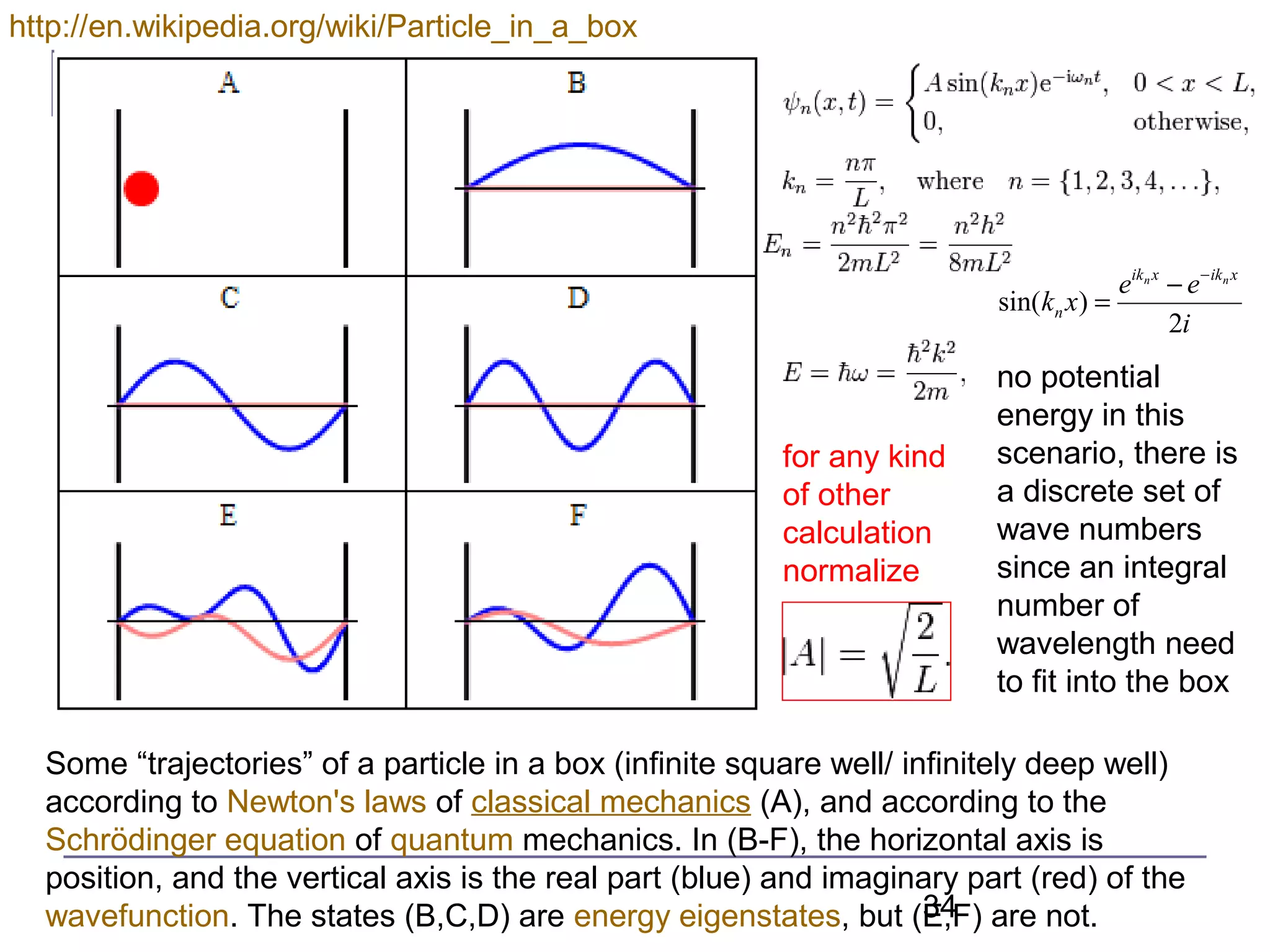
Illustration of energy eigenstates for a particle in a box, contrasting classical and quantum mechanical behavior.
Introductory discussion on Bohr’s correspondence principle as it relates to quantum systems.
Importance of normalization in wave functions to ensure valid probability calculations in quantum physics.
Continued examination of Bohr's principles in quantum mechanics and their applications.
Discussion on the nature of stationary wave functions and their implications for quantum states.
Summary of historical milestones related to quantum mechanics and its development.
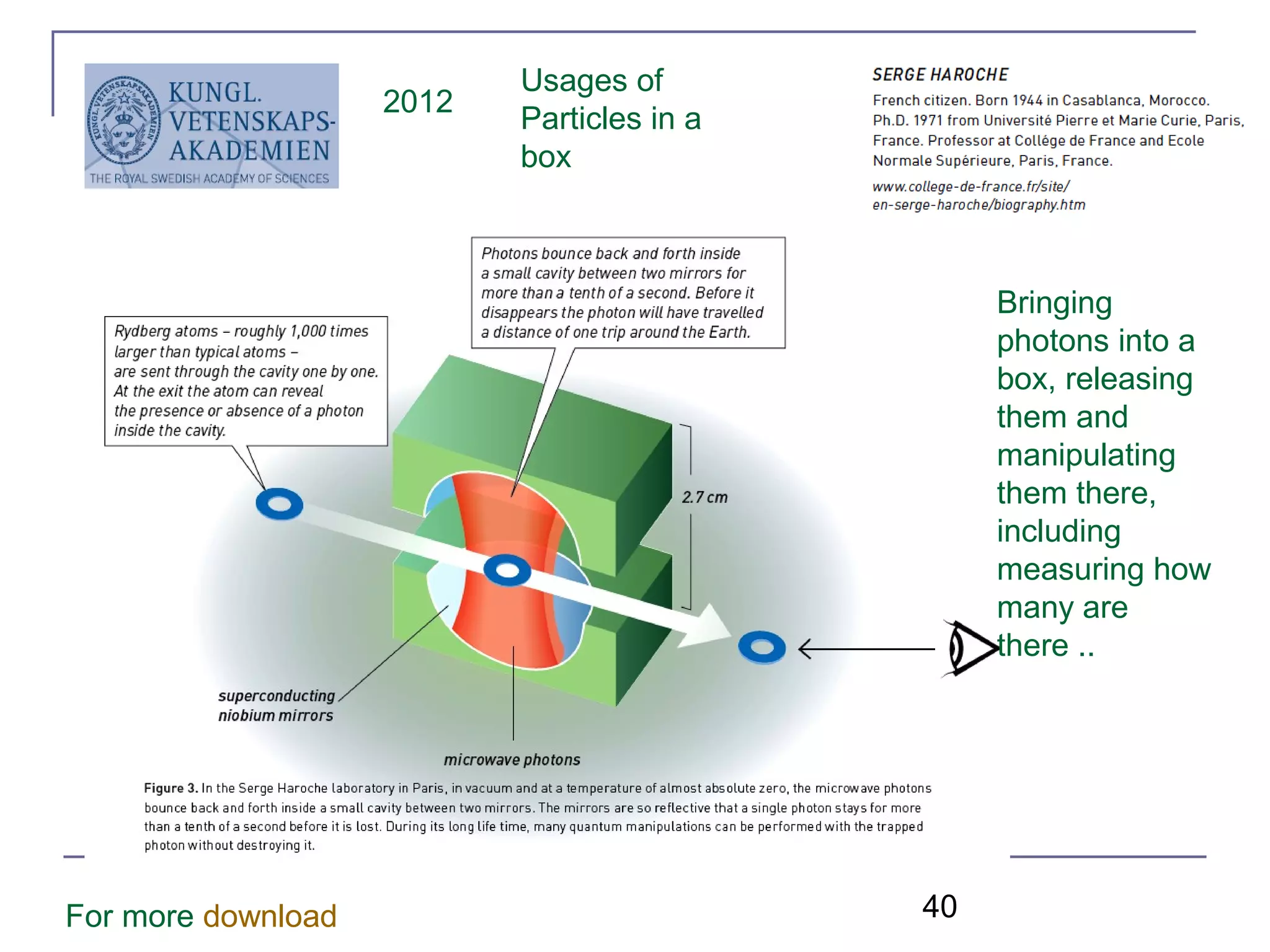
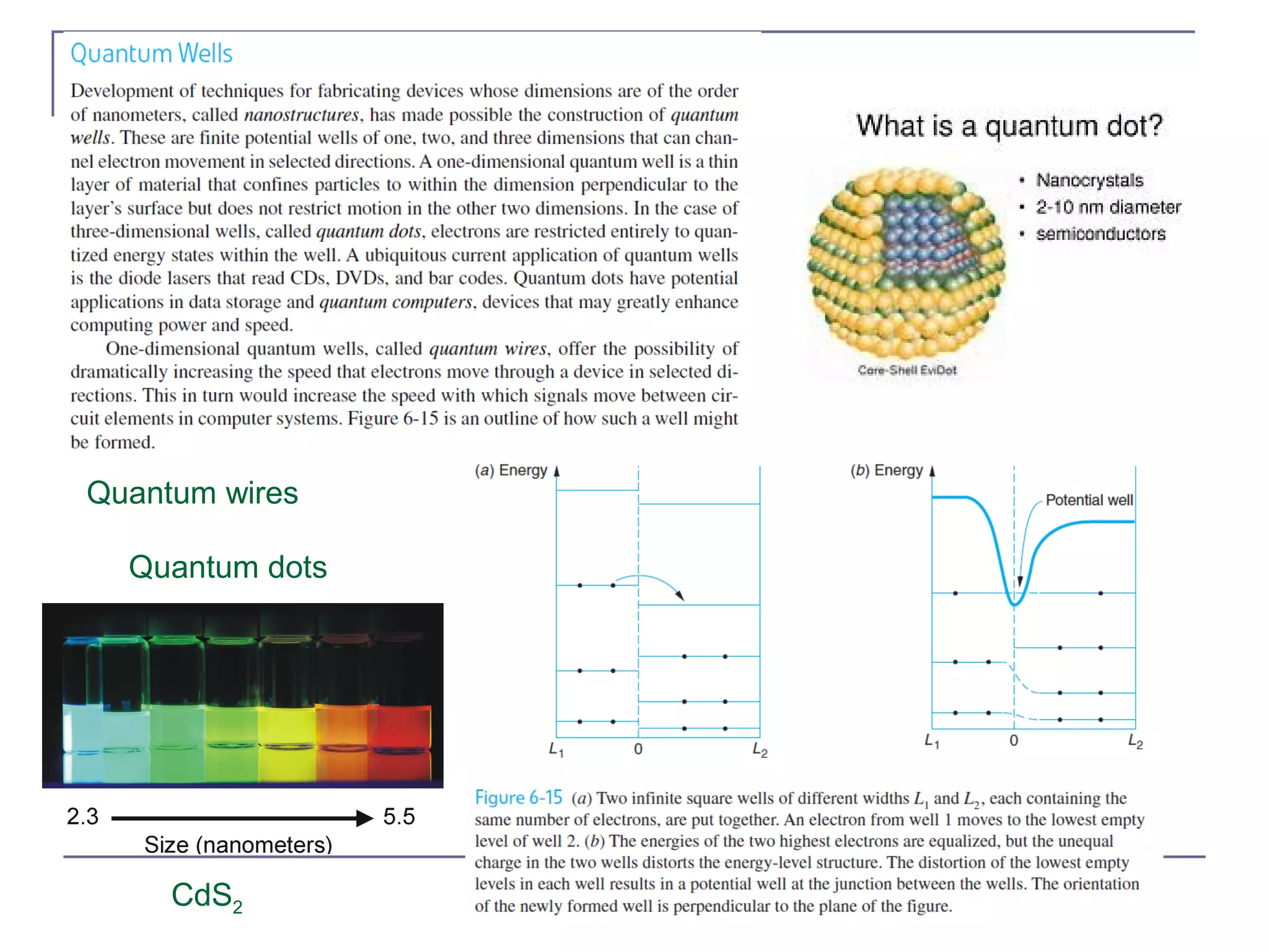
Overview of practical applications of quantum mechanics, particularly in particle manipulation.
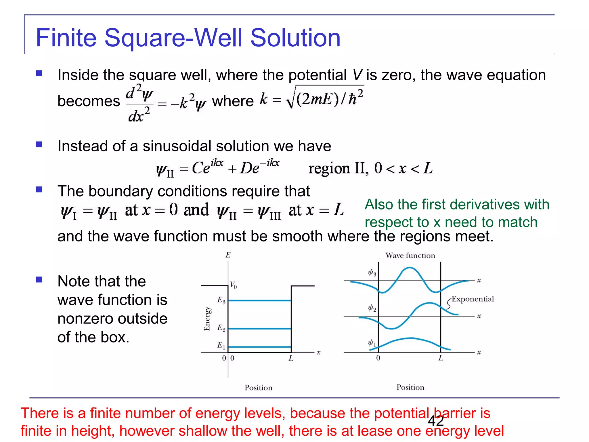
Introduction to the finite square-well potential and its significance in quantum mechanics.
Analysis of wave solutions within the finite square well and boundary matching conditions.
Discussion on penetration depth and its correlation with quantum probabilities outside potential wells.
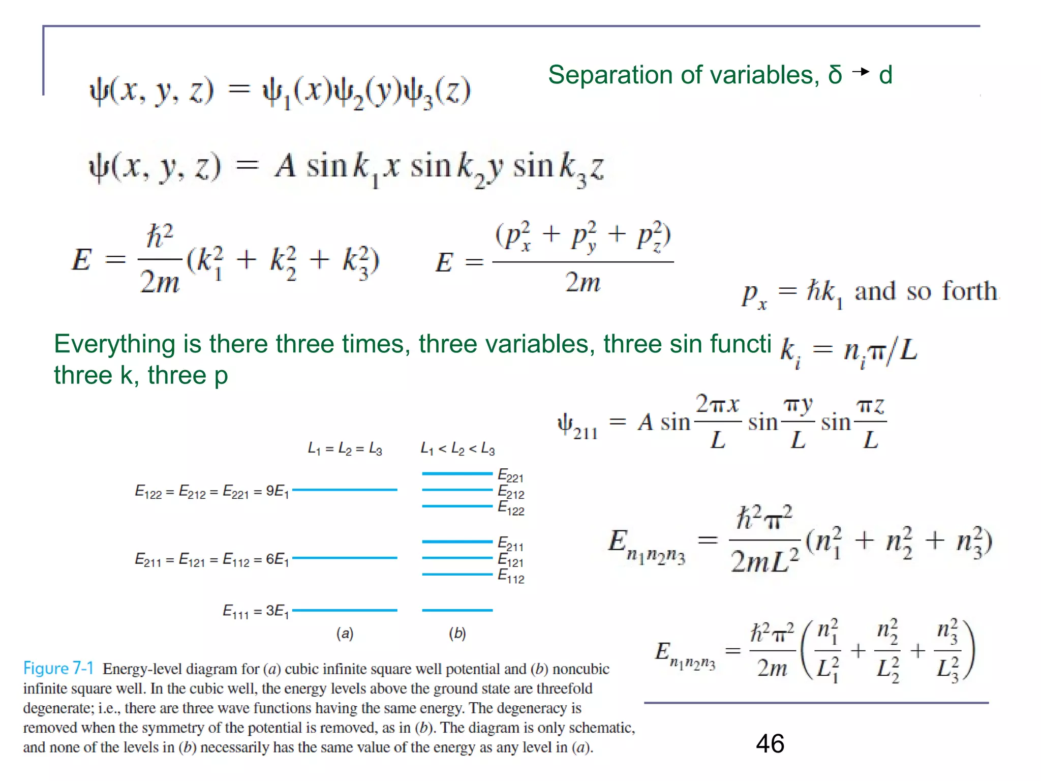
Introduction to the three-dimensional Schrödinger wave equation and its implications in physics.
Examination of multi-variable separations required for solving complex quantum systems.
Analysis of energy state degeneracy in three-dimensional quantum systems and its symmetry properties.
Exploration of the implications of high symmetry in quantum systems, affecting degeneracy.
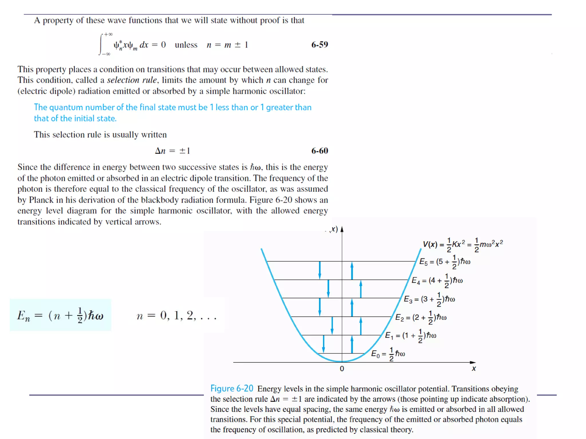
Understanding simple harmonic oscillators and their applications in various physical systems.
Examines energy levels and wave functions in parabolic potentials and contrasting properties.
Describes contrasting behavior of quantum probabilities inside a parabolic well.
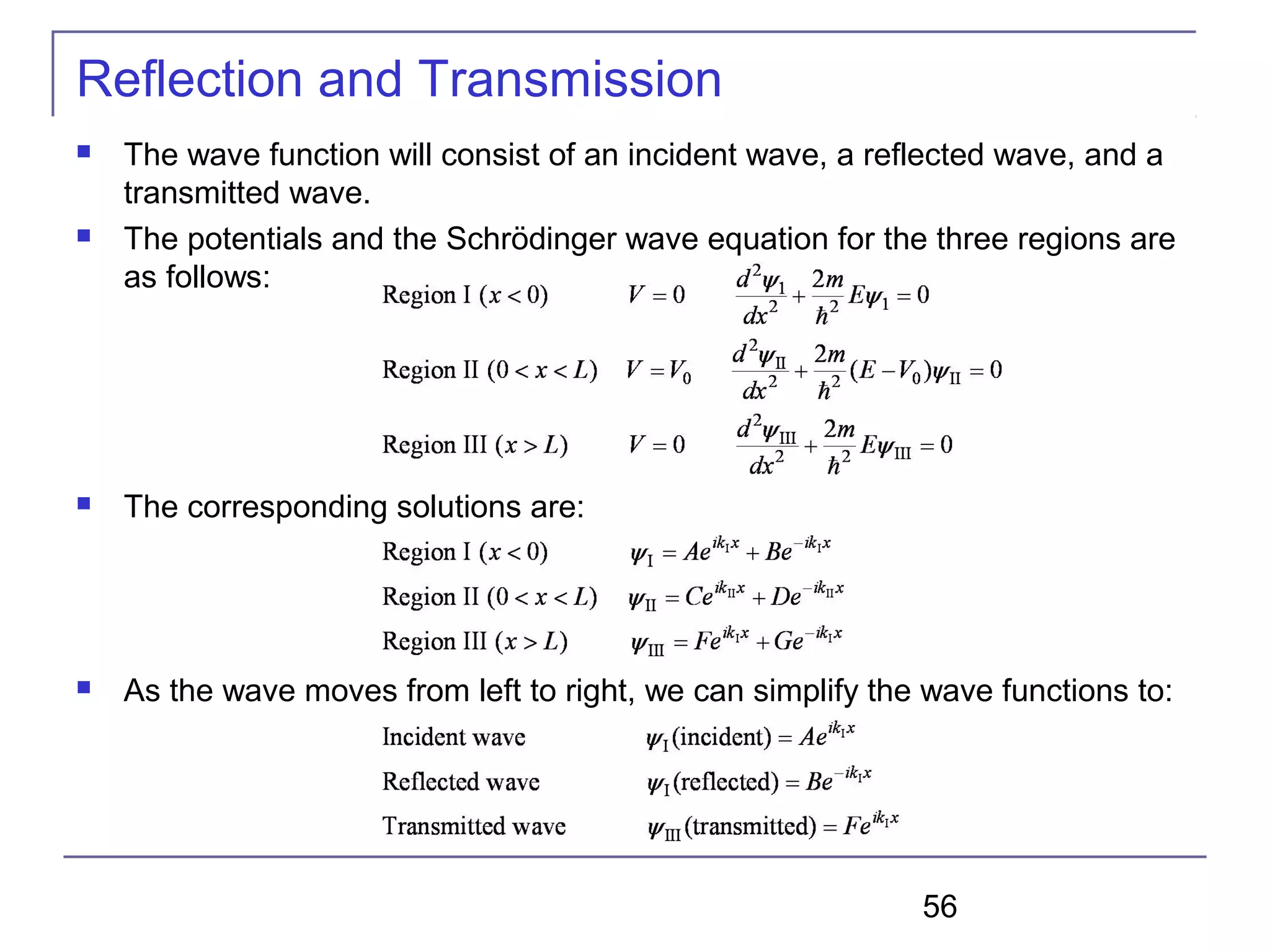
Introduction to potential barriers in quantum mechanics and the roles of reflection and transmission.
Analysis of wave behavior at potential barriers, including reflection and transmission probabilities.
Exploration of probabilities associated with reflection and transmission in quantum systems.
Examines particle dynamics through potential wells versus barriers within quantum frameworks.
Describes the phenomenon of tunneling in quantum mechanics, detailing its significance.
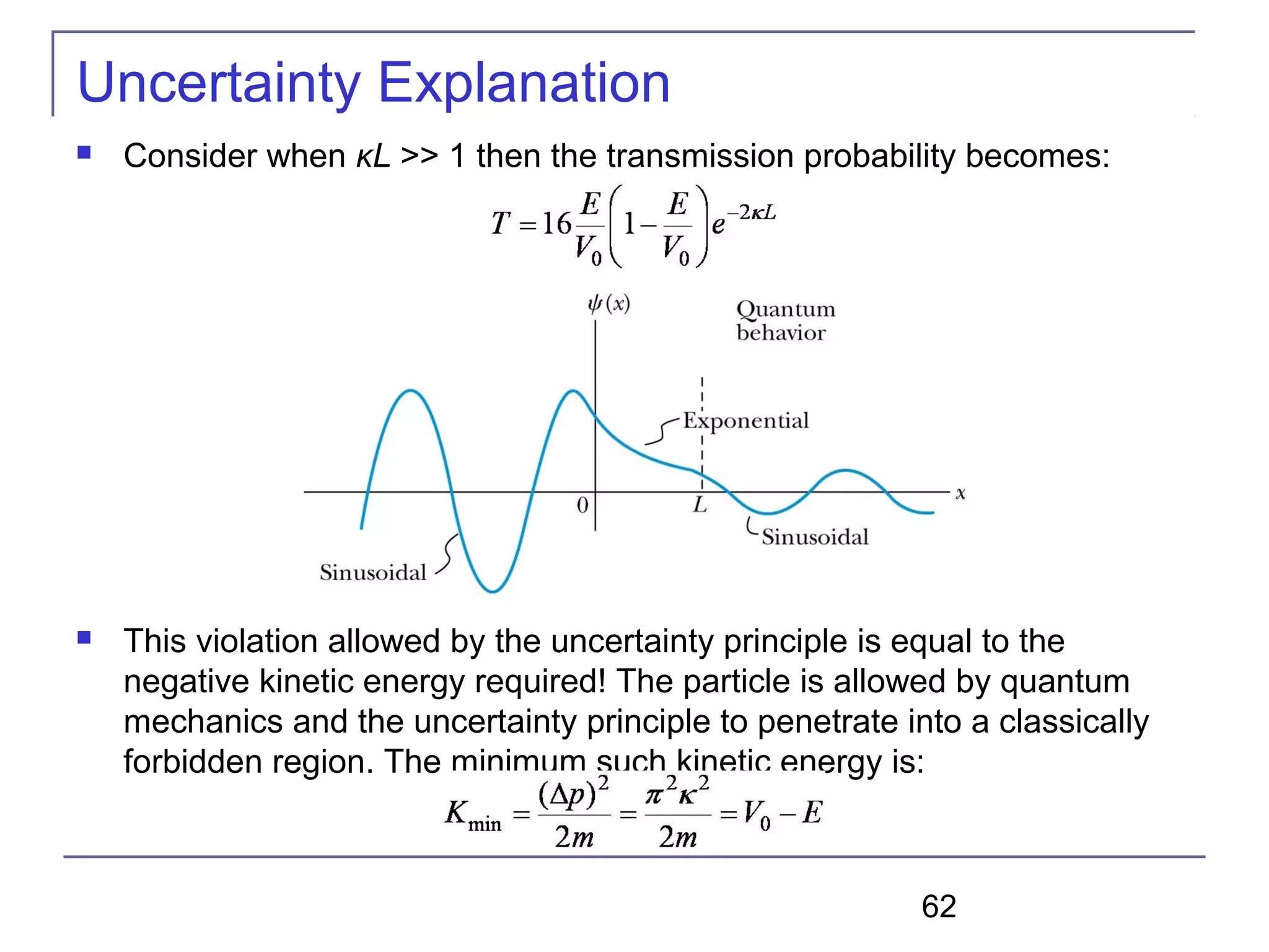
Discussion of the uncertainty principle in quantum mechanics and its implications for energy measurements.
Examination of tunneling and uncertainty principles illustrating quantum behavior.
Analogies between optical phenomena and quantum tunneling, illustrating foundational principles.
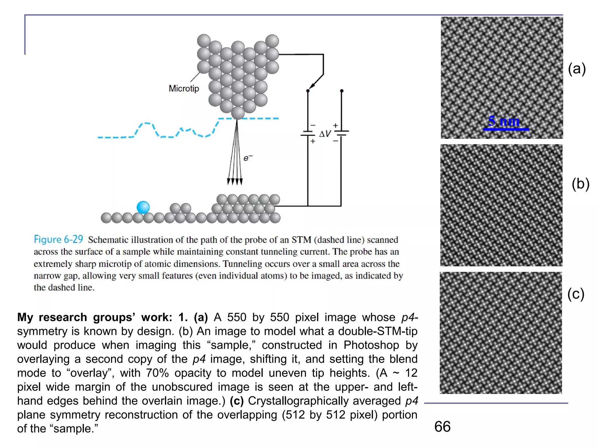
Presentation of research contributions regarding quantum image modeling and symmetry in physics.
Discussion on radioactivity and related quantum principles discovered post-1896.
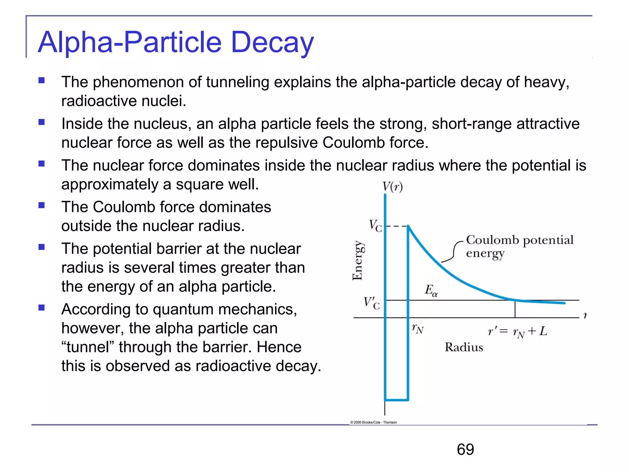
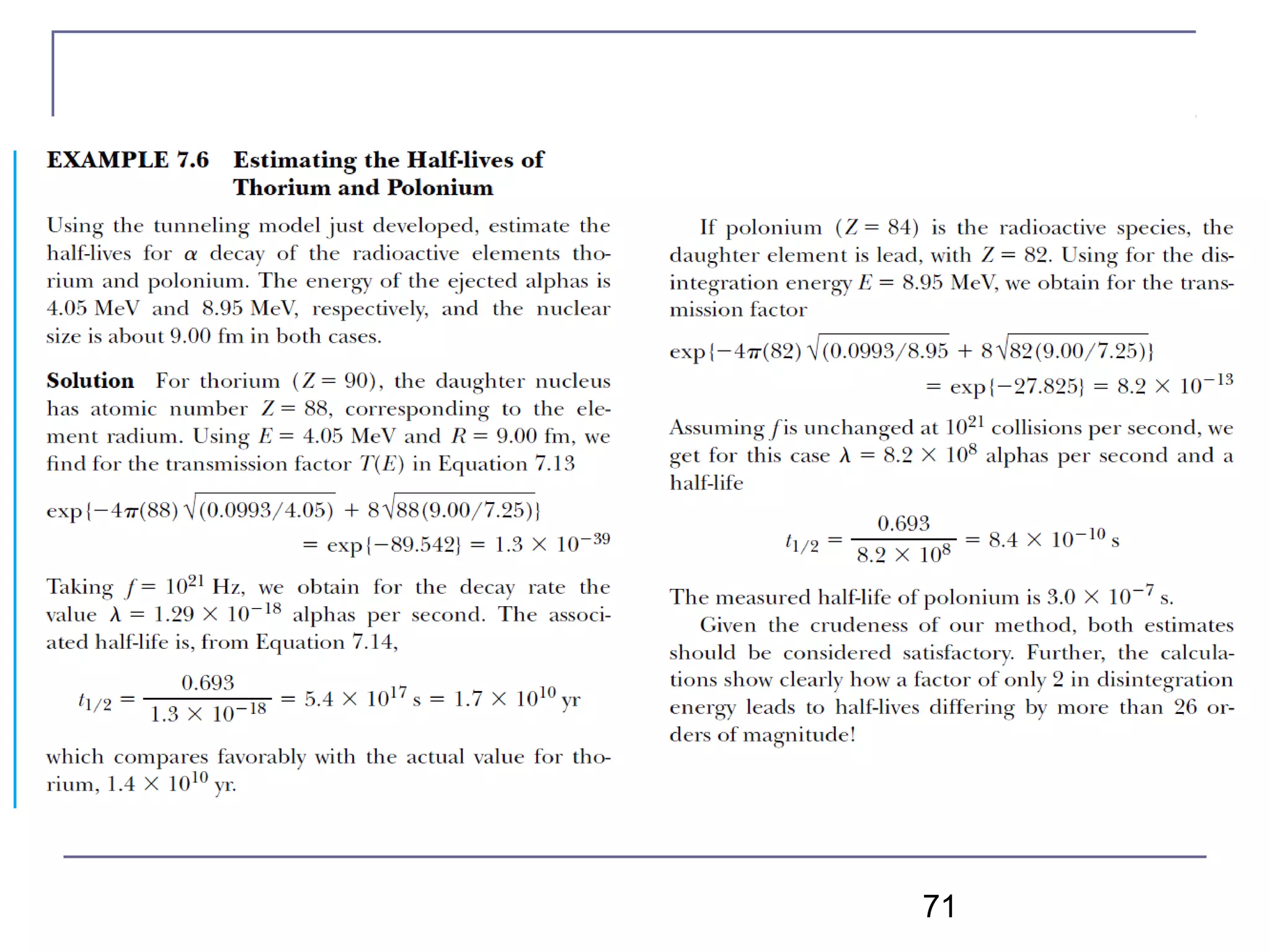
Using the tunneling phenomenon to explain alpha-particle decay in radioactive nuclei.
1
6.0 Partialdifferentials
6.1 The Schrödinger Wave Equation
6.2 Expectation Values
6.3 Infinite Square-Well Potential
6.4 Finite Square-Well Potential
6.5 Three-Dimensional Infinite-Potential Well
6.6 Simple Harmonic Oscillator
6.7 Barriers and Tunneling in some books an
extra chapter due to its technical importance
CHAPTER 6
Quantum Mechanics IIQuantum Mechanics II
I think it is safe to say that no one understands quantum mechanics. Do not keep saying to
yourself, if you can possibly avoid it, “But how can it be like that?” because you will get
“down the drain” into a blind alley from which nobody has yet escaped. Nobody knows how it
can be like that.
- Richard Feynman
2.
2
2
),( yxyxf =
2
.}
),(
{
),(
x
y
yxf
y
yxf
consx=
∂
∂
=
∂
∂
=
yx
x
yxf
x
yxf
consy 2}
),(
{
),(
. =
∂
∂
=
∂
∂
= y
x
yxf
xx
yxf
consy 2}
),(
{
),(
.2
2
=
∂
∂
∂
∂
=
∂
∂
=
0}
),(
{
),(2
.2
=
∂
∂
∂
∂
=
∂
∂
=consx
y
yxf
yy
yxf
yyxf
y
yxf
x
yxf 2),((),(),( 2
2
2
2
2
=
∂
∂
+
∂
∂
=∇
d→∂
y will often be time t for 1D wave functions
axax
eae
dx
d
⋅=)( iaxiax
eiae
dx
d
⋅=)(
axaax
dx
d
cos)(sin ⋅=
axaax
dx
d
sin)(cos ⋅−=
θθθ
sincos ie i
−=−
θθθ
sincos iei
+=
0}
),(
{
),(
.2
2
=
∂
∂
∂
∂
=
∂
∂
=consx
y
yxf
yy
yxf
3.
3
Modern Physics
waves or
particles?
Howcome
they are
characteristic
of atoms?
How come we can’t
derive this from
Maxwellian waves?
then applications,
PH 312
the correct theory of matter
at lastJ.J. Thompson (1987) electron
5
Plane wave forelectric
field vector
Light “wavicals” are special, obey the time dependent
Helmholtz (wave) equation
As we also know from special relativity
A light wave is its own probability density wave, idea by Einstein
fc λ=
λ
hkp ==
6.
6
Loved his pipe,wine, and many mistresses = a really great physicist, kind of
started biophysics with his booklet “What is life?”
left the top theoretical physics position in all of Germany (at Berlin University)
for Ireland on his own account in 1938 disgruntled by stupid German policies,
his mother was English, …Republic of Ireland remained neutral during WWII
7.
7
6.1. The SchrödingerWave Equation
The Schrödinger wave equation in its time-dependent form for a
particle of energy E moving in a potential V in one dimension is
The extension into three dimensions is
where is an imaginary number.
The statement is in both cases that operators act on the
wave function, V = V(x,t) in the first equation for 1D, V =
V(x,y,z,t) in the second equation for 3D
Equivalent to time dependent
Helmholtz (wave) equation,
which can be derived from
Newton’s force laws, BUT
Schrödinger equation cannot be
derived from anything else !!!
m = mass of electron
8.
8
Comparison of Classicaland Quantum
Mechanics
Newton’s second law and Schrödinger’s wave equation are
both differential equations.
Newton’s second law can be derived from the Schrödinger
wave equation, so the latter is the more fundamental – cannot
be derived from anything else.
Classical mechanics only appears to be more precise because
it deals with macroscopic phenomena. The underlying
uncertainties in macroscopic measurements are just too small
to be significant, the un-correctable systematic rest error that is
due to the uncertainty principle is too small to be noticed for
heavy objects
am
dt
xdm
dtdt
xdm
dt
vdm
dt
pdF
⋅=⋅=
⋅
⋅=⋅== 2
Non-relativistically, m is constant and taken out of
the differential
9.
9
Divide by thewave function, what do you get?
Total energy = kinetic energy + potential energy in operator
form, i.e. total energy is conserved, we ignore rest energy
and special relativity, always need to make sure that
particles move with v < 0.01c or better 1
/α ≈ 1
/137
while there can be undetected energy fluctuations within the uncertainty limit,
wave particle duality is taken care of by the i, i.e. going complex, into Hilbert
space
),( txE Ψ⋅=
Eigenfunctions of total energy En solve Schroedienger equation, En are
eigenvalues (you may remember algebra of matrices, solving linear systems of equations)
),( txE Ψ⋅=
10.
10
The potential
energy function
doesnot vary in
space and time,
it’s a constant,
either zero or any
value
Free particle wave function solves the
Schrödinger equation with a constant
potential, can be set zero
11.
11
It’s simply aconsequence of the linearity of
the Schrödinger equation, if two wave
functions are solutions to it, the sum and
difference between the two is also a solution.
Modern physics is not about cats in boxes, but all kinds of tiny
tiny particles in their natural environment, before we look we do
not know in which of many allowed states a particle is in, so we
do look, i.e. collapse the wave function into a probability
density and calculate all that is knowable by expectation values
(with the help of operators on the wavefunction)
12.
12
Free particle solutionof the Schrödinger wave
equation, harmonic/plane matter wave, V = 0 or constant
The wave function for a plane wave
which describes a wave moving in the x direction to the right from
minus infinity to plus infinity (left it you change the sign). In general
the amplitude (A) may also be complex. Out of the sum of infinitely
many different plane matter waves, we can create wave packets,
just as we did for classical waves earlier
Wave functions are also not restricted to being real. All traveling
matter waves are complex. Note that the sin term has an imaginary
number in front of it. Only physically measurable quantities must be
real. These include the probability of finding the particle someplace
(either sometimes or all the time), momentum, energy, anything you
want to know
If V = 0 and not constant, it is no longer a free particle, then we need
to normalize, setting the scale for all measurements by operators
13.
13
Normalization and Probability
The probability P(x) dx of a particle being between x and x + dx
was given in the equation
The probability of the particle being between x1 and x2 is given
by
The wave function must also be normalized so that the
probability of the particle being somewhere on the x axis is 1.
Since the only things we are allowed to know are all calculated from the wave
function for a particular physical scenario V(x,t) function, normalization sets the
scale
Compare previous chapter !!!
14.
14
Need to fulfillthis
condition,
Ψ(x,t) and Ψ*(x,t) both
needs to have the
same prefactor that is
the reciprocal value of
the integral when
multiplied
It is going to be 1/Sqrt
whatever the integral
comes to
something finite
1
_
1*
_
1 =•Ψ•Ψ∫
∞
∞−
dx
finitesomethingfinitesomething
since Schrödinger
equation is linear, a
prefactor on both sides
changes nothing
15.
15
try to normalizethe wave function for a free
particle
∞
No big deal, just a useful model, superposing of infinitely many plane
waves with the right properties leads to the wave packet that we need to
normalize in order to set the physical scale right
What
does this
mean?
Probability of fining the particle is in each finite unit segment identical
and finite, adding all of these unit segments together gives infinity – so
the particle is everywhere at the same time, better one does not know
where it is at all
But
no longer apply,
definite E and p
here we have a ∆E again
16.
16
Properties of validwave functions
I. Boundary conditions, to make the mathematics
work
1) In order to avoid infinite probabilities, the wave function must be finite
everywhere.
2) In order to avoid multiple values of the probability, the wave function
must be single valued.
3) For finite potentials, the wave function and its derivative must be
continuous. This is required because the second-order derivative term
in the wave equation must be single valued. (There are exceptions to
this rule when V is infinite.)
4) In order to normalize the wave functions, they must approach zero as x
approaches infinity.
Wave functions that do not posses these mathematical
properties do not correspond to physically realizable
circumstances.
= 1 for normalization
17.
17
Properties of validwave functions II
II. Boundary condition, to bring the physics in
Every problem has its specific wave function (that sure
needs to get the maths of the Schrödinger equation right)
it all depends on the potential energy function, the physics
of the problem to be solved is encoded there
we need a function, not a vector so instead of force we use
potential energy
Fxk
kx
dx
d
−==)
2
(
2
2
)()(
2
kx
xUxV ==
e.g. potential energy
function of a spring, does
not depend on time
Hooke’s law in
Newton’s formulation
V1 can be set zero
∫ ⋅−=−=∆
2
1
12 xdFVVV
gradient of potential
energy function = - force
18.
18
Time-Independent Schrödinger Wave
Equation
The potential in many cases will not depend explicitly on time.
The dependence on time and position can then be separated in the
Schrödinger wave equation. Let ,
which yields:
Now divide by the wave function:
The left side depends only on time, and the right side depends only on
spatial coordinates. Hence each side must be equal to a constant. The
time dependent side is
What might this B possibly be? given the
fact that the Schrödinger equation is a
statement on the conservation of total
energy, which is constant in a stationary
state
19.
19
We integrateboth sides and find:
where C is an integration constant that we may choose to be 0. Therefore
This determines f to be
This is known as the time-independent Schrödinger wave equation, and it is a
fundamental equation in quantum mechanics.
Time-Independent Schrödinger Wave
Equation Continued
Dimensional analysis of
the exponent leads to E !
What else could B possibly
be? given the fact that the
Schrödinger equation is a
statement on the
conservation of total energy
In order to do this, f(t) needs
to be eigen function
20.
20
Stationary State
Thewave function can be written as:
Whenever the potential energy function is not time dependent
The probability density becomes:
The probability distributions are constant in time. This is a standing
wave phenomena that is called the stationary state.
ω⋅= E So whenever you see circular frequency omega, you can also
think total energy divided by h-bar
λ
hkp == So whenever you see the wave number, you can also
think linear momentum divided by h-bar
Remember when you see
E think ω and vice versa
21.
21
6.2: Expectation Values,what one will measure on
average is derived from correct wave function for a problem
The expectation value is the expected result of the average of
many measurements of a given quantity. The expectation value
of x is denoted by <x>
Any measurable quantity for which we can calculate the
expectation value is called a physical observable. The
expectation values of physical observables (for example,
position, linear momentum, angular momentum, and energy)
must be real, because the experimental results of
measurements are real.
The average value of x is
3 3 4 4
22.
22
Continuous Expectation Values
We can change from discrete to
continuous variables by using the
probability P(x,t) of observing the
particle at a particular x and t.
Using the wave function, the
expectation value is:
The expectation value of any
function g(x) for a normalized wave
function:
x and g(x) are operators !!!, x could also have been in the middle of
conjugant complex wave function times wave function as it the rule
for all operators
23.
23
Momentum Operator
Tofind the expectation value of p, we first need to
represent p in terms of x and t. Consider the derivative
of the wave function of a free particle with respect to x:
With k = p / ħ we have
This yields
This suggests we define the momentum operator as
.
The expectation value of the momentum is
λ
hkp ==
24.
24
The positionx is its own operator as seen above.
The time derivative of the free-particle wave function is
Substituting ω = E / ħ yields
The energy operator is
The expectation value of the energy is
Position and Energy Operators
ω⋅= E
25.
25
For anything youwant to know, there is an operator, the procedure is always
the same to get the information out of the wave function that represents your
problem, just let the correct operator loose on it, it’s that simple
26.
26
Only a veryfew operators are fundamental
If you need an operator, make it up from the classical
physics equation by replacing x, p, E(t) with their
operators
The new operator will have the same functional relationship
for the x, p, E(t) operators as the classical physics
equation,
example kinetic energy operator
m
p
mvKE
22
1
2
2
==
][ˆ xxx ==
2
222
2
)()(
2
1
2
ˆˆ][
xmx
i
x
i
mm
p
KEEKKE op
∂
∂
⋅−=
∂
∂
−⋅
∂
∂
−⋅====
27.
27
Some expectation valuesare sharp some
others fuzzy
Since there is scatter in the actual positions
(x), the calculated expectation value will
have an uncertainty, fuzziness (Note that x
is its own operator.)
][ˆ xxx ==
][ˆ xxx =>≠<
Normalizing condition, note its effect !
28.
28
Some expectation valuesare sharp some
others fuzzy, continued I
For any observable, fuzzy or not
If not fuzzy, ΔQ = 0
Because <Q2
>= <Q>2
x may as well stand
for any kind of
operator Q
29.
29
Some expectation valuesare sharp some
others fuzzy, continued II
Eigen values of operators are always sharp (an actual – physical
- measurement may give some variation in the result, but the
calculation gives zero fuzziness
Say Q is the Hamiltonian operator A wave function that solves this
equation is an eigenfunction of this
operator, E is the corresponding
eigenvalue, apply this operator
twice and you get E2
– which sure is
the same as squaring to result of
applying it once (E)
So if the potential energy operator acts to confine a particle of mass m, we
will have a discrete set of stationary states with total energies, E1, E2, …
][ˆ][ˆ)( VVUUxU ====
31
6.3: Infinite Square-WellPotential
The simplest such system is that of a particle trapped in a box with infinitely
hard walls that the particle cannot penetrate. This potential is called an
infinite square well and is given by
Clearly the wave function must be zero where the potential
is infinite,
there will be infinitely many En eigenvaules with their matching eigenfunctions
Where the potential is zero inside the box, the Schrödinger wave
equation becomes where .
The general solution is .
Note that this wave function is real because we are considering a
standing wave, that is the sum of two moving waves
i
ee
xk
xikxik
n
nn
2
)sin(
−
−
=
B = 0, as just the sin term will do
λ
π2=k
n
nk
λ
π2=
32.
32
Physical boundary condition
Boundary conditions of the potential dictate that the wave function must
be zero at x = 0 and x = L. This yields valid solutions for integer values of
n such that kL = nπ.
The wave function is now
We normalize the wave function
The normalized wave function becomes
These functions are identical to those obtained for a vibrating string with
fixed ends.
33.
33
Quantized Energy
Thequantized wave number now becomes
Solving for the energy yields
Note that the energy depends on the integer values of n. Hence the
energy is quantized and nonzero.
The special case of n = 1 is called the ground state energy.
There is an infinite number of energy levels, because the potential barrier
is infinitely high
Ground
state
energy,
zero point
energy,
there is
no n = 0
34.
34
Some “trajectories” ofa particle in a box (infinite square well/ infinitely deep well)
according to Newton's laws of classical mechanics (A), and according to the
Schrödinger equation of quantum mechanics. In (B-F), the horizontal axis is
position, and the vertical axis is the real part (blue) and imaginary part (red) of the
wavefunction. The states (B,C,D) are energy eigenstates, but (E,F) are not.
http://en.wikipedia.org/wiki/Particle_in_a_box
no potential
energy in this
scenario, there is
a discrete set of
wave numbers
since an integral
number of
wavelength need
to fit into the box
for any kind
of other
calculation
normalize
i
ee
xk
xikxik
n
nn
2
)sin(
−
−
=
36
Normalization, to setthe
scale of a wave function
if we had not used a normalized wave
function, the probability of finding the
particle in the box would not be unity, and
we would not have gotten our 81.8% result
40
2012
Usages of
Particles ina
box
Bringing
photons into a
box, releasing
them and
manipulating
them there,
including
measuring how
many are
there ..
For more download
41.
41
6.4: Finite Square-WellPotential
The finite square-well potential is
The Schrödinger equation outside the finite well in regions I and III is
or using
yields . Considering that the wave function must be zero at
infinity, the solutions for this equation are
Note the importance of the sign in the Schroedinger equation
42.
42
Inside thesquare well, where the potential V is zero, the wave equation
becomes where
Instead of a sinusoidal solution we have
The boundary conditions require that
and the wave function must be smooth where the regions meet.
Note that the
wave function is
nonzero outside
of the box.
Finite Square-Well Solution
There is a finite number of energy levels, because the potential barrier is
finite in height, however shallow the well, there is at lease one energy level
Also the first derivatives with
respect to x need to match
43.
43
Penetration Depth
Thepenetration depth is the distance outside the potential well where
the probability significantly decreases. It is given by
It should not be surprising to find that the penetration distance that
violates classical physics is proportional to Planck’s constant.
45
The wavefunction must be a function of all three spatial coordinates.
We begin with the conservation of energy
Multiply this by the wave function to get
Now consider momentum as an operator acting on the wave
function. In this case, the operator must act twice on each
dimension. Given:
The three dimensional Schrödinger wave equation is
6.5: Three-Dimensional Infinite-Potential Well
First slide in this chapter
46.
46
Separation of variables,δ d
Everything is there three times, three variables, three sin functions,
three k, three p
47.
47
Degeneracy
Analysis ofthe Schrödinger wave equation in three dimensions
introduces three quantum numbers that quantize the energy.
A quantum state is degenerate when there is more than one
wave function (eigen function) for a given energy (eigen value).
Degeneracy results from particular symmetry properties of the
potential energy function that describes the system. A perturbation of
the potential energy can remove the degeneracy.
For a cubic box
50
6.6: Simple HarmonicOscillator
Simple harmonic oscillators describe many physical situations: springs,
diatomic molecules and atomic lattices.
Consider the Taylor expansion of a potential function:
Redefining the minimum potential and the zero potential, we have
Substituting this into the wave equation:
Let and which yields .
51.
51
Parabolic Potential Well
If the lowest energy level is zero, this violates the uncertainty principle.
The wave function solutions are where Hn(x) are Hermite
polynomials of order n.
In contrast to the particle in a box, where the oscillatory wave function is a
sinusoidal curve, in this case the oscillatory behavior is due to the polynomial,
which dominates at small x. The exponential tail is provided by the Gaussian
function, which dominates at large x.
52.
52
Analysis of theParabolic Potential Well
The energy levels are given by
The zero point energy is called the Heisenberg
limit:
Classically, the probability of finding the mass is
greatest at the ends of motion and smallest at the
center (that is, proportional to the amount of time
the mass spends at each position).
Contrary to the classical one, the largest probability
for this lowest energy state is for the particle to be
at the center.
54
6.7: Barriers andTunneling
Consider a particle of energy E approaching a potential barrier of height V0 and the
potential everywhere else is zero.
We will first consider the case when the energy is greater than the potential
barrier.
In regions I and III the wave numbers are:
In the barrier region we have
56
Reflection and Transmission
The wave function will consist of an incident wave, a reflected wave, and a
transmitted wave.
The potentials and the Schrödinger wave equation for the three regions are
as follows:
The corresponding solutions are:
As the wave moves from left to right, we can simplify the wave functions to:
57.
57
Probability of Reflectionand Transmission
The probability of the particles being reflected R or transmitted T is:
The maximum kinetic energy of the photoelectrons depends on the
value of the light frequency f and not on the intensity.
Because the particles must be either reflected or transmitted we have:
R + T = 1.
By applying the boundary conditions x → ±∞, x = 0, and x = L, we arrive
at the transmission probability:
Notice that there is a situation in which the transmission probability is 1.
58.
58
Potential Well
Considera particle passing through a potential well region rather than through a
potential barrier.
Classically, the particle would speed up passing the well region, because K = mv2
/ 2 =
E + V0.
According to quantum mechanics, reflection and transmission may occur, but the
wavelength inside the potential well is smaller than outside. When the width of the
potential well is precisely equal to half-integral or integral units of the wavelength, the
reflected waves may be out of phase or in phase with the original wave, and
cancellations or resonances may occur. The reflection/cancellation effects can lead to
almost pure transmission or pure reflection for certain wavelengths. For example, at the
second boundary (x = L) for a wave passing to the right, the wave may reflect and be
out of phase with the incident wave. The effect would be a cancellation inside the well.
59.
59
Tunneling
Now weconsider the situation where classically the particle does not have
enough energy to surmount the potential barrier, E < V0.
The quantum mechanical result, however, is one of the most remarkable features
of modern physics, and there is ample experimental proof of its existence. There
is a small, but finite, probability that the particle can penetrate the barrier and even
emerge on the other side.
The wave function in region II becomes
The transmission probability that
describes the phenomenon of tunneling is
61
x
where ħ =h/2π, and σx, σp are the standard deviations of position (r) and momentum
Funny Quantum energy bank: you can get a
no interest loan ΔE for a certain time Δt as
long as ΔE Δt < h
62.
62
Uncertainty Explanation
Considerwhen κL >> 1 then the transmission probability becomes:
This violation allowed by the uncertainty principle is equal to the
negative kinetic energy required! The particle is allowed by quantum
mechanics and the uncertainty principle to penetrate into a classically
forbidden region. The minimum such kinetic energy is:
64
Analogy with WaveOptics
If light passing through a glass prism reflects from an
internal surface with an angle greater than the critical
angle, total internal reflection occurs. However, the
electromagnetic field is not exactly zero just outside
the prism. If we bring another prism very close to the
first one, experiments show that the electromagnetic
wave (light) appears in the second prism The situation
is analogous to the tunneling described here. This
effect was observed by Newton and can be
demonstrated with two prisms and a laser. The
intensity of the second light beam decreases
exponentially as the distance between the two prisms
increases.
66
My research groups’work: 1. (a) A 550 by 550 pixel image whose p4-
symmetry is known by design. (b) An image to model what a double-STM-tip
would produce when imaging this “sample,” constructed in Photoshop by
overlaying a second copy of the p4 image, shifting it, and setting the blend
mode to “overlay”, with 70% opacity to model uneven tip heights. (A ~ 12
pixel wide margin of the unobscured image is seen at the upper- and left-
hand edges behind the overlain image.) (c) Crystallographically averaged p4
plane symmetry reconstruction of the overlapping (512 by 512 pixel) portion
of the “sample.”
(c)
(a)
(b)
5 nm
68
There is alsoradioactivity (from 1896 onwards):
electrons and other particles, e.g. alpha
particles, (we now know nuclei of He, two
proton + two neutrons) come out of the atoms of
certain elements
end of the second part of this course, nuclear
physics
69.
69
Alpha-Particle Decay
Thephenomenon of tunneling explains the alpha-particle decay of heavy,
radioactive nuclei.
Inside the nucleus, an alpha particle feels the strong, short-range attractive
nuclear force as well as the repulsive Coulomb force.
The nuclear force dominates inside the nuclear radius where the potential is
approximately a square well.
The Coulomb force dominates
outside the nuclear radius.
The potential barrier at the nuclear
radius is several times greater than
the energy of an alpha particle.
According to quantum mechanics,
however, the alpha particle can
“tunnel” through the barrier. Hence
this is observed as radioactive decay.