How to make a conditional column chart in Excel
•Download as PPTX, PDF•
6 likes•8,362 views

This is an easy way to add a quick display to Executive Dashboard Template in Excel.

Recommended
More Related Content
What's hot
What's hot (20)
Viewers also liked
Viewers also liked (20)
Similar to How to make a conditional column chart in Excel
Similar to How to make a conditional column chart in Excel (20)
Recently uploaded
Recently uploaded (20)
How to make a conditional column chart in Excel
- 2. Conditional charts can be very effective in your Executive dashboard presentations
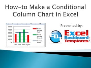
- 3. As you build a Microsoft Excel dashboard, you might want to highlight your data that exceeds your Key Performance Indicators (KPIs) as well as those that do not. Many businesses use Averages as a KPI breakpoint in their executive dashboards. In Excel, use any Key Performance Indicator line to highlight your dashboard data. More powerful than the average line would be to highlight when the data is above or below the line by conditionally changing the column colors in the Excel chart. ◦ If the data point is above the average then have excel automatically color that column green. ◦ If the data point is below the average, color that column red.
- 4. In a previous post, “How-to Hide a Zero Pie Chart Slice or Stacked Column Chart Section, you saw how to use the Excel Function NA() to hide a slice of pie or a part of a stacked column chart. Now let’s use the NA() Function to hide columns in a chart.
- 5. If you chart a range of data like this that uses the NA() function in an Excel Column Chart: It will look like this with the #N/A values not being plotted in the chart at all. That way we can make a different chart series for every color or condition that we want to display.
- 6. 1) Make a new chart area for the Conditional Columns and change the data into 3 series. ◦ One for values below average. ◦ One for values equal to or above average ◦ One for the average line. ◦ Use the NA() Function in your formulas for this setup.
- 7. 2) Chart the 3 series. When you chart the 3 series, you will not see any columns that are equal to #N/A. The #N/A values are hidden and that is how to change the colors on the chart conditionally.
- 8. 3) Change the average data series to a line chart:
- 9. 4) Change the colors of each series to suit your needs. For instance, you can change the below average series = Red, and the above average = Green. Format the rest of the chart and series and clean up the presentation. Now you are done!
- 10. Create a separate data area for the chart that will create what we want. In E2, put in =A2 for your X-Axis Labels. In H2, put in =$C$2. In F2, put in the formula: =IF($B2>=$H$2,$B2,NA()) ◦ What this formula does is that it compares the value in B2 to the average per month. If B2 is greater or equal to the average, then the formula will put in the number from B2 and if it is less than the average it will put in #N/A in the worksheet cell. When we chart these series, the #N/A will not show columns for these values.
- 11. Highlight and Copy E2:H2 then paste from E2 to H5
- 12. Highlight the new chart data range - E1:H5 and then Click on Insert Ribbon and Select a Column Chart (2D).
- 13. Right Click on the Average Data Series and Select Change Series Chart Type to a Line Chart or Left click on the Average Series and then choose the Change Chart Type from the Design Ribbon.
- 14. Right Click on the Above Average Data Series and Select Format Data Series… from the menu or Left click on the Average Series and choose the Change Chart Type from the Design Ribbon.
- 15. Change the Above Average Series to Plot on the Secondary Axis. Now your data may look strange because the second vertical axis min and max are probably not be the same as the primary vertical axis. But don’t worry, we will fix this issue in a future step.
- 16. Select the Fill Sub Menu and Change the Fill option to a Solid Fill and then choose Green as the color.
- 17. Change the Below Average Series Red color by selecting the series from the chart without closing down the Format Data Series dialog box.
- 18. Change the Average Series Line color to Blue by selecting the series from the chart without closing down the Format Data Series dialog box.
- 19. Now you will see that your data looks off. That is because the Primary and Secondary min and max values are not the same for each axis. If you delete the Secondary Vertical Axis, the data and columns will line up to the right levels. Select the Secondary Vertical Axis and Delete press the delete key or right click on it and choose Delete from the menu.
- 20. Now we are done and here is what your final Excel Dashboard chart will looks like:
- 21. Video Tutorial ◦ If you would like to see a video demonstration of this technique in Excel Chart building, please visit our YouTube Channel at this link: ◦ http://www.youtube.com/watch?v=PDA8mkabmTQ&context=C365ce01ADOEgsToPD skKurwZJjUzhYGOXDcQAuCmQ Free Sample Download Tutorial File ◦ We have a FREE download sample tutorial file that has detailed instructions and the base formulas that you can try on your own at this URL: ◦ http://www.exceldashboardtemplates.com/?p=891 (Link at the bottom) Thanks for viewing this presentation! ◦ Please visit our blog and let us know if you found this helpful by posting a comment and don’t forget to sign up for the RSS Feed. That way you are sure to get the most current Excel Dashboard Tutorial. ◦ http://www.exceldashboardtemplates.com/