This document summarizes recommender systems, focusing on collaborative filtering techniques. It discusses how recommender systems help with information overload by matching users with relevant items. Collaborative filtering is introduced as a technique that seeks to predict user preferences based on other similar users' ratings. The document then covers various collaborative filtering algorithms like neighborhood models, latent factor models using matrix factorization, and extensions like adding biases and temporal dynamics. It concludes by discussing hybrid methods and providing references for further reading.

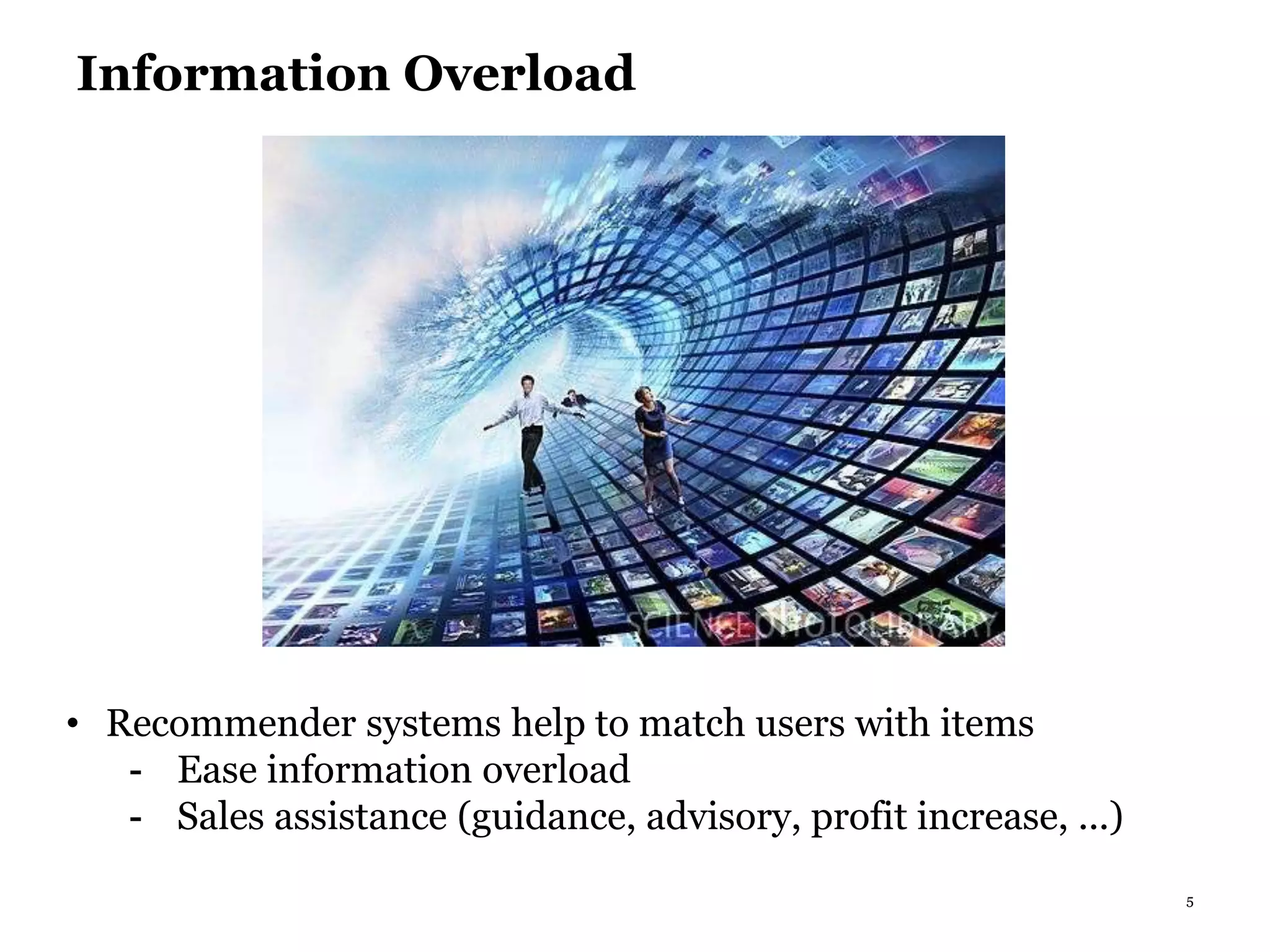
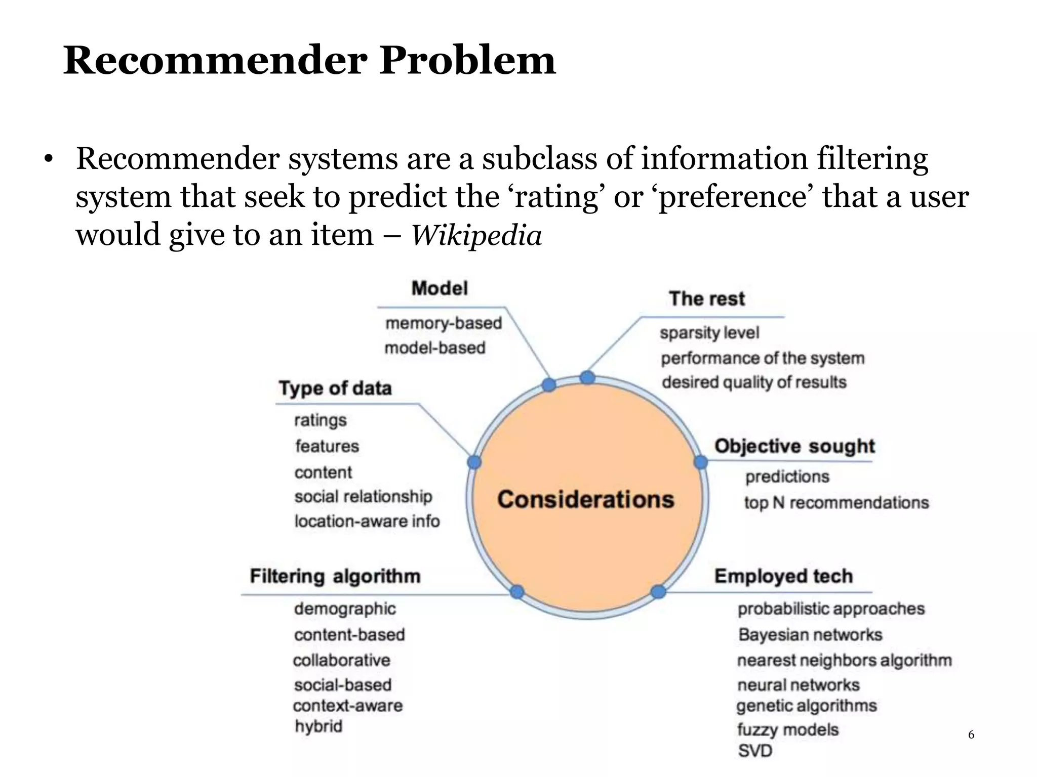
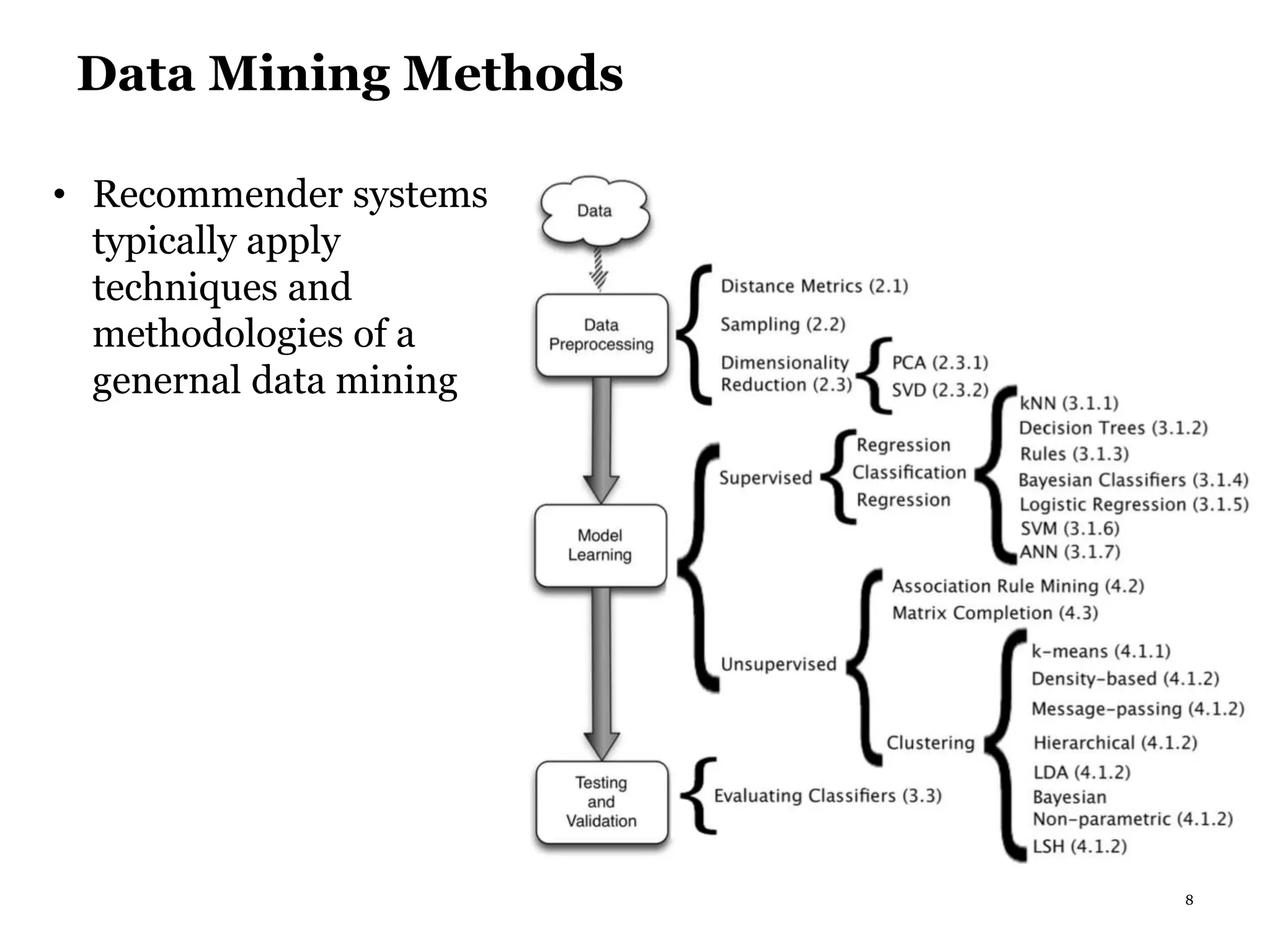
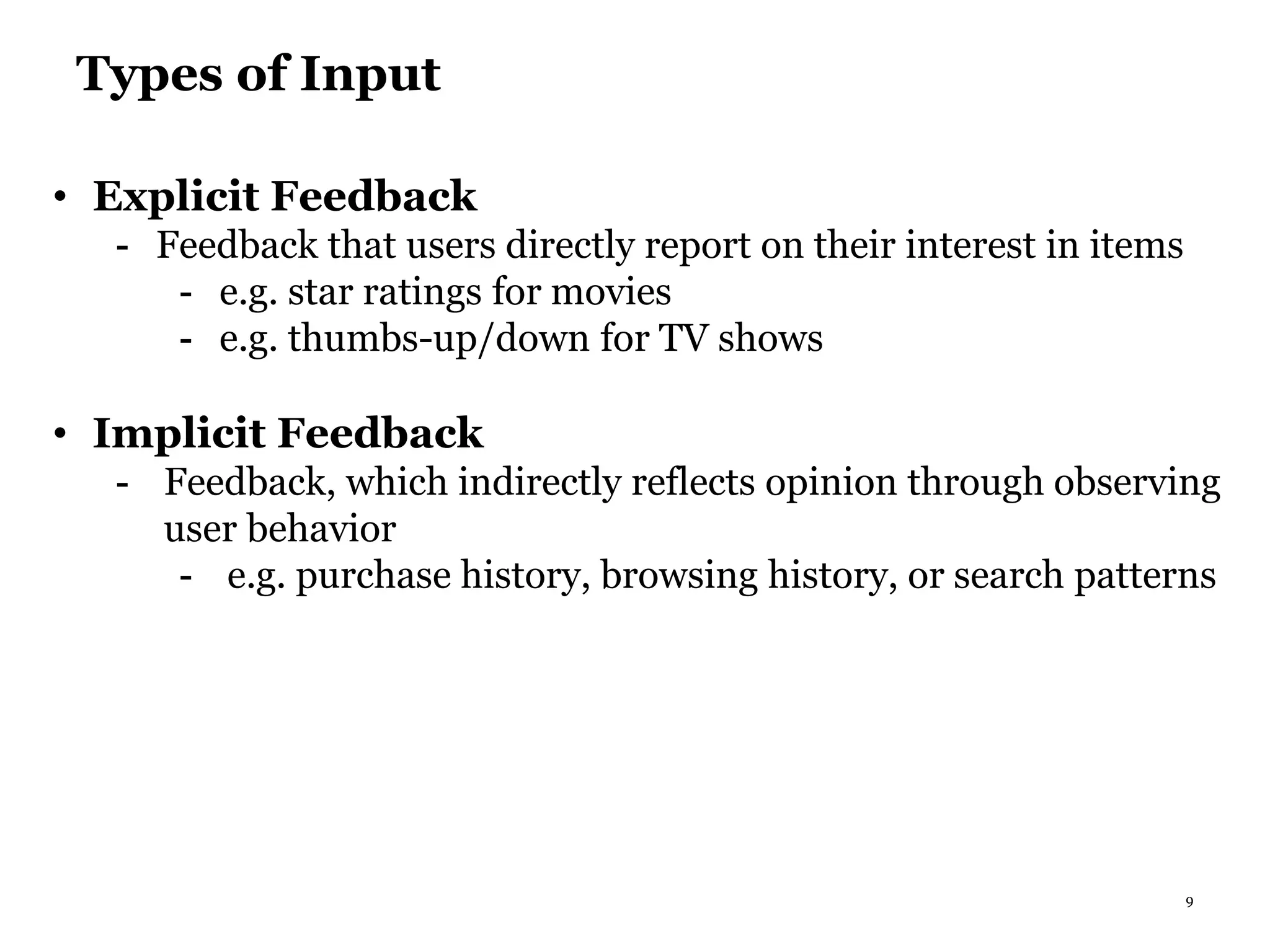
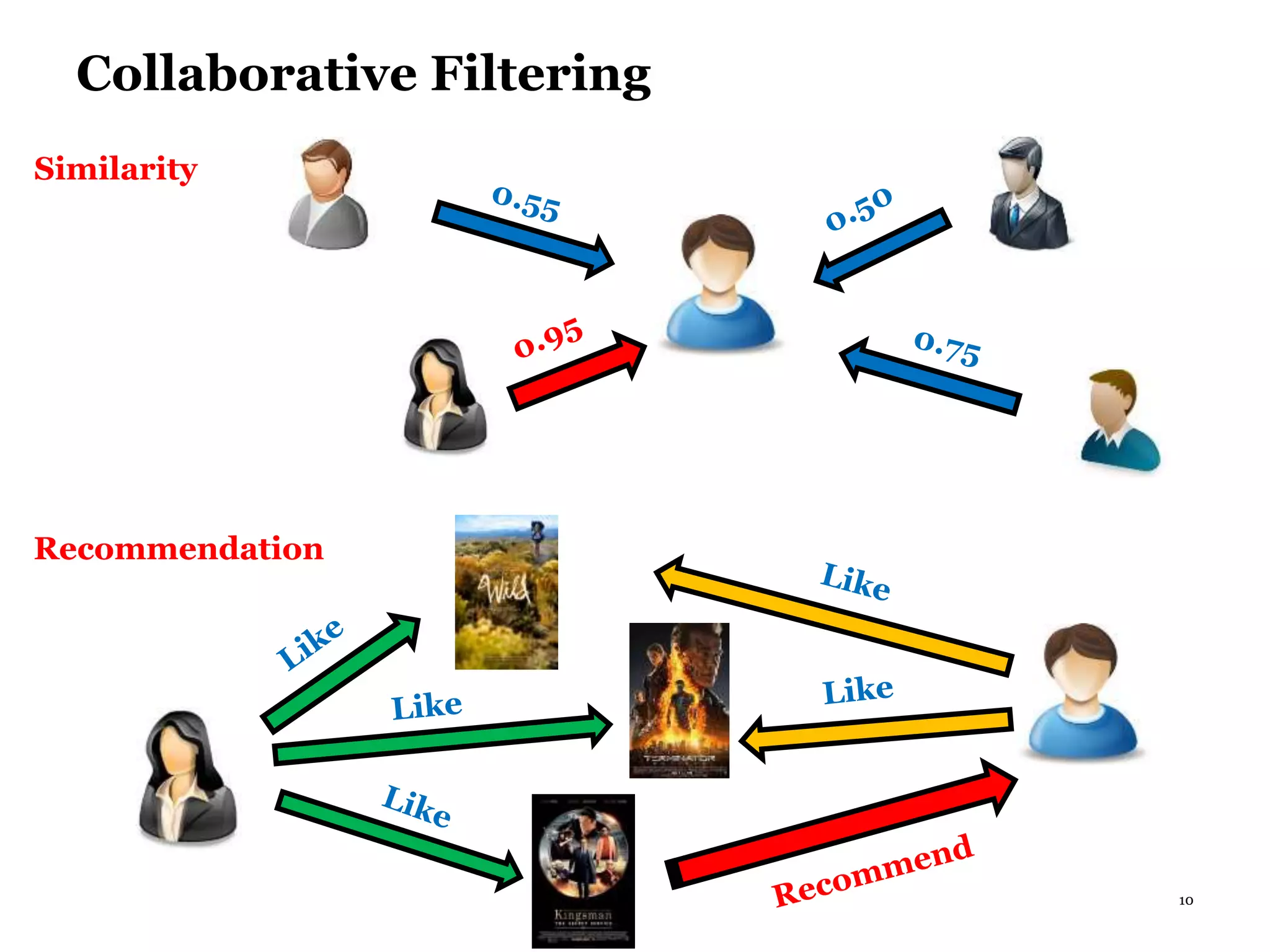
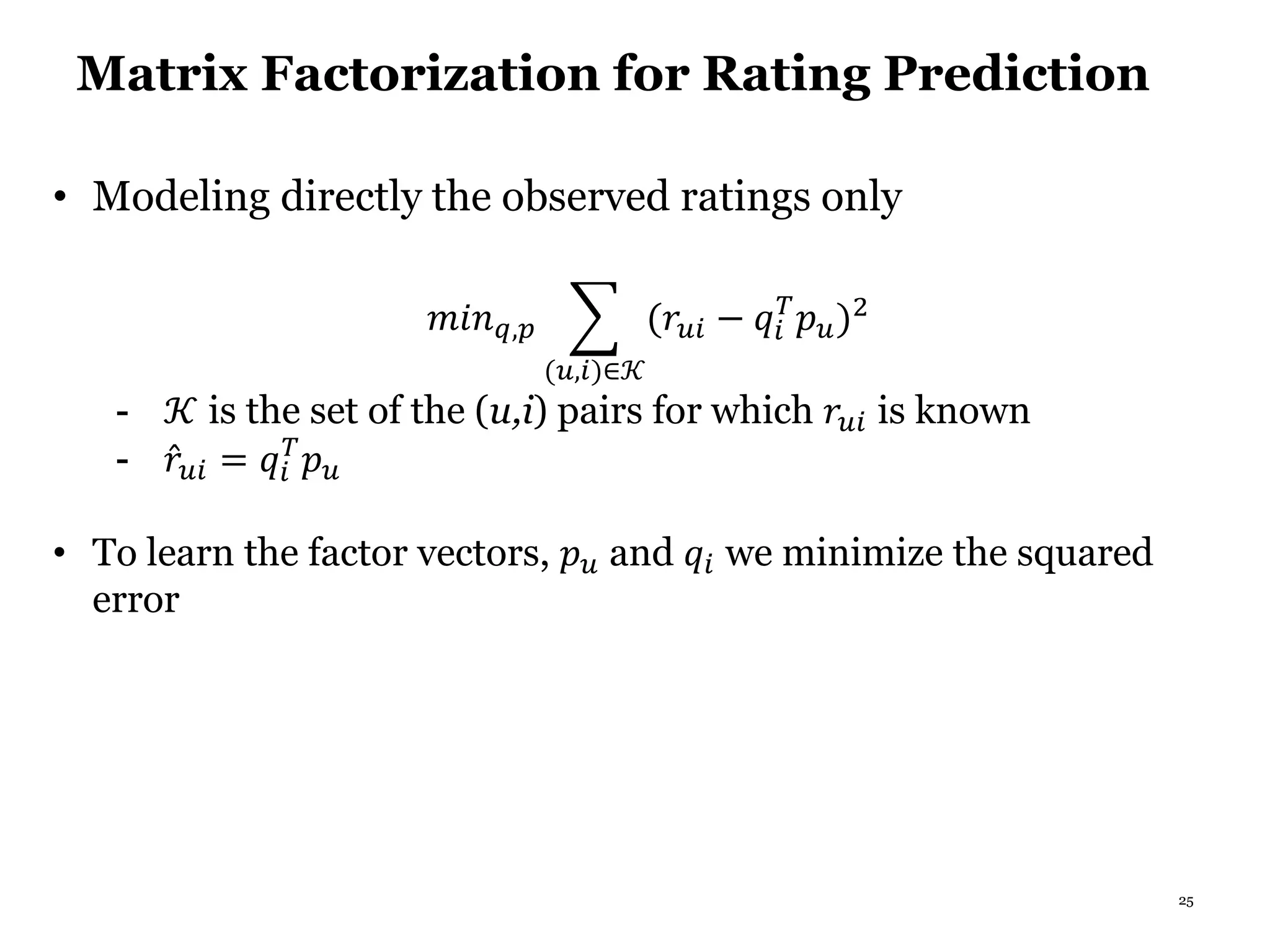
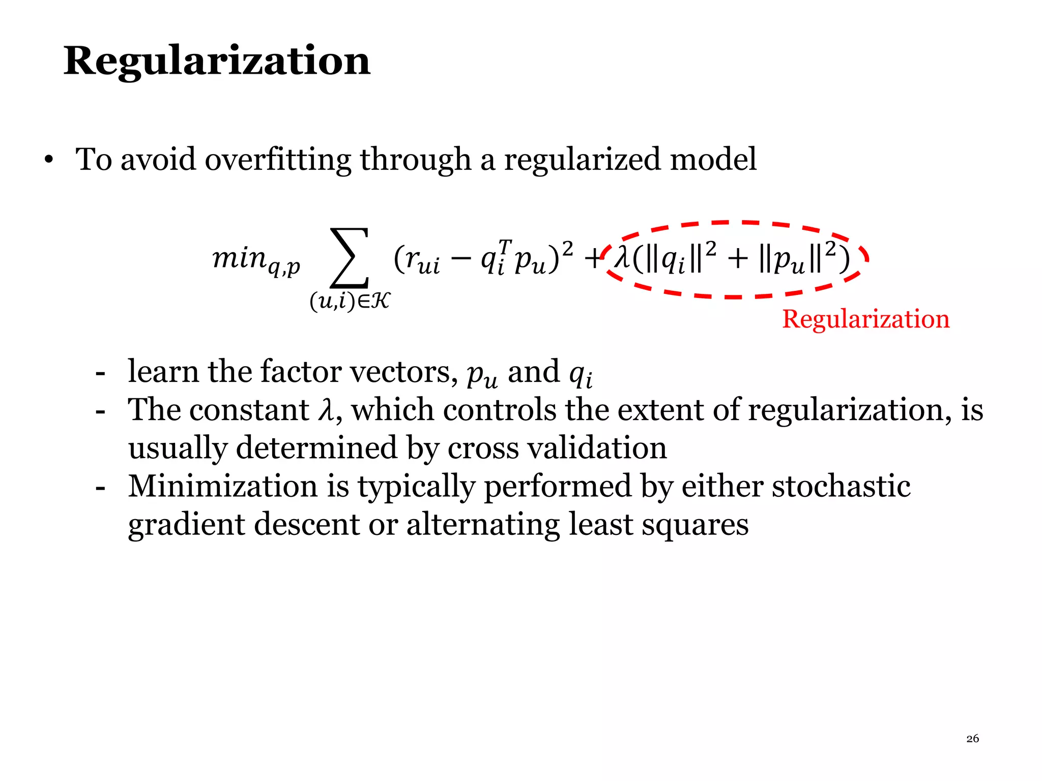
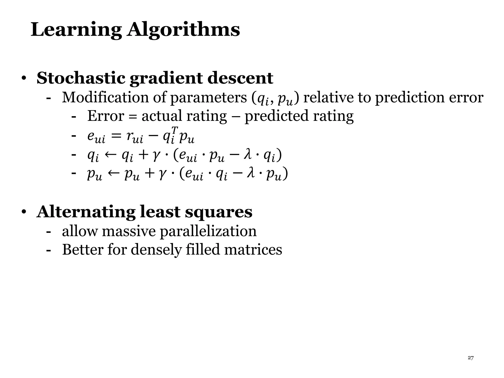
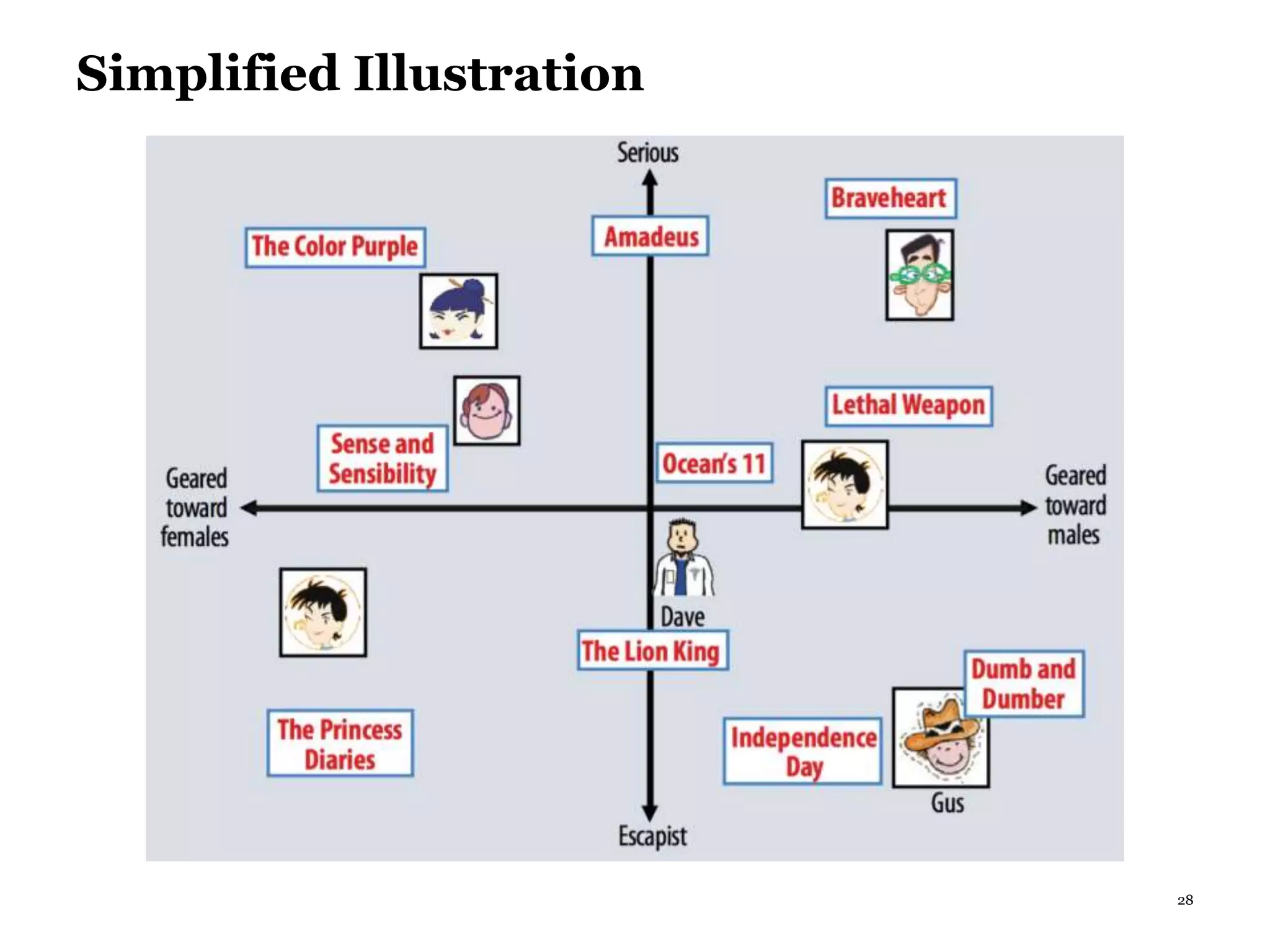
1. Recommender Systems:
Backgrounds &
Advances in Collaborative Filtering
1
Changsung Moon
Department of Computer Science
North Carolina State University

2. 2
Amazon.com

3. 3
Netflix

4. 4
The Long Tail
Source: http://www.wired.com/2004/10/tail/

5. 5
Information Overload
• Recommender systems help to match users with items
- Ease information overload
- Sales assistance (guidance, advisory, profit increase, ...)

6. 6
Recommender Problem
• Recommender systems are a subclass of information filtering
system that seek to predict the ‘rating’ or ‘preference’ that a user
would give to an item – Wikipedia

7. 7
Recommenders Trends

8. 8
Data Mining Methods
• Recommender systems
typically apply
techniques and
methodologies of a
genernal data mining

9. 9
Types of Input
• Explicit Feedback
- Feedback that users directly report on their interest in items
- e.g. star ratings for movies
- e.g. thumbs-up/down for TV shows
• Implicit Feedback
- Feedback, which indirectly reflects opinion through observing
user behavior
- e.g. purchase history, browsing history, or search patterns

10. 10
Collaborative Filtering
Similarity
Recommendation

11. 11
Pros of Collaborative Filtering
• requires minimal knowledge engineering efforts
• needs not consider content of items
• produces good enough results in most cases
• Serendipity of results

12. 12
Challenges for Collaborative Filtering
• Sparsity
- Usually the vast majority of ratings are unknown
- e.g. 99% of ratings are missing in Netflix data
• Scalability
- Nearest neighbor techniques require computation that grows
with both the number of users and the number of items
• Cold Start Problem
- New items and new users can cause the cold-start problem, as
there will be insufficient data for CF to work accurately

13. 13
Challenges for Collaborative Filtering
• Popularity Bias
- tends to recommend popular items
• Synonyms
- Same or very similar items having different names or entries
- Topic modeling like LDA could solve this by grouping
different words belonging to the same topic
• Shilling Attacks
- People may give positive ratings for their own items and
negative ratings for their competitors

14. 14
Content-based Recommendation
• Based on information about item itself, usually keywords or
phrases occurring in the item
• Similarity between two content items is measured by similarity
associated with their term vectors
• User’s profile can be developed by analyzing set of content the
user interacted with
• enables you to compute the similarities between a user and an
item
Similar

15. 15
Pros/Cons of Content-based Approach
• Pros
- No need for data on other users: No cold-start or sparsity
- able to recommend to users with unique tastes
- able to recommend new and unpopular items
- provides explanations by listing content features
• Cons
- In certain domains (e.g., music, blogs and videos), it is
complicated to generate the features for items
- difficult to implement serendipity
- Users only receive recommendations that are very similar
to items they liked or prefered

16. 16
Hybrid Methods
• Weighted
- Outputs from several techniques are combined with different
weights
• Switching
- Depending on situation, the system changes from one
technique to another
• Mixed
- Outputs from several techniques are presented at the same
time
• Cascade
- The output from one technique is used as input of another that
refines the results

17. 17
Hybrid Methods
• Feature Combination
- Features from different recommendation sources are
combined as input to a single technique
• Feature Augmentation
- The output from one technique is used as input features to
another
• Meta-level
- The model learned by one recommender is used as input to
another

18. 18
Two Main Techniques of CF
• Neighborhood Approach
- Relationships between items or between users
• Latent Factor Models
- Transforming both items and users to the same latent factor
space
- Characterizing both items and users on factors inferred from
user feedback
- pLSA
- neural networks
- Latent Dirichlet Allocation
- Matrix factorization (e.g. SVD-based models)
- ...

19. 19
Latent Factor Models
• find features that describe the characteristics of rated objects
• Item characteristics and user preferences are described with
numerical factor values
Action Comedy

20. 20
Latent Factor Models
• Items and users are associated with a factor vector
• Dot-product captures the user’s estimated interest in the item
𝑟𝑢𝑖 = 𝑞𝑖
𝑇
𝑝 𝑢
- Each item i is associated with a vector 𝑞𝑖 ∈ ℝ 𝑓
- Each user u is associated with a vector 𝑝 𝑢 ∈ ℝ 𝑓
• Challenge – How to compute a mapping of items and users to
factor vectors?
• Approaches
- Matrix Factorization Models
- e.g. Singular Value Decomposition (SVD)

21. 21
SVD
• R: 𝑁 × 𝑀 matrix (e.g., N users, M movies)
• U: 𝑁 × 𝑘 matrix (e.g., N users, k factors)
• 𝚺: 𝑘 × 𝑘 diagonal matrix with k largest eigenvalues
• V 𝒕
: 𝑘 × 𝑀 matrix (e.g., k factors, M movies)

22. 22
SVD
5 5 1
5 4 2
1 2 2
1 3 5
𝑓1 𝑓2
-0.44-0.63
-0.23-0.60
0.25-0.25
0.83-0.43
𝑓1
𝑓2
-0.67-0.62
-0.03-0.52
-0.41
0.85
𝑓1
𝑓2
𝑓1 𝑓2
010.96
4.390
R U
𝑽 𝒕
𝚺

23. 23
SVD
𝑓1
𝑓2

24. 24
SVD - Problems
• Conventional SVD has difficulties due to high portion of missing
values in the user-item ratings matrix
• Imputation to fill in missing ratings
- Imputation can be very expensive as it significantly increases
the amount of data
- Inaccurate imputation might distort the data

25. 25
Matrix Factorization for Rating Prediction
• Modeling directly the observed ratings only
𝑚𝑖𝑛 𝑞,𝑝
(𝑢,𝑖)∈𝒦
(𝑟𝑢𝑖 − 𝑞𝑖
𝑇
𝑝 𝑢)2
- 𝒦 is the set of the (u,i) pairs for which 𝑟𝑢𝑖 is known
- 𝑟𝑢𝑖 = 𝑞𝑖
𝑇
𝑝 𝑢
• To learn the factor vectors, 𝑝 𝑢 and 𝑞𝑖 we minimize the squared
error

26. 26
Regularization
• To avoid overfitting through a regularized model
𝑚𝑖𝑛 𝑞,𝑝
(𝑢,𝑖)∈𝒦
(𝑟𝑢𝑖 − 𝑞𝑖
𝑇
𝑝 𝑢)2
+ 𝜆( 𝑞𝑖
2
+ 𝑝 𝑢
2
)
- learn the factor vectors, 𝑝 𝑢 and 𝑞𝑖
- The constant 𝜆, which controls the extent of regularization, is
usually determined by cross validation
- Minimization is typically performed by either stochastic
gradient descent or alternating least squares
Regularization

27. 27
Learning Algorithms
• Stochastic gradient descent
- Modification of parameters (𝑞𝑖, 𝑝 𝑢) relative to prediction error
- Error = actual rating – predicted rating
- 𝑒 𝑢𝑖 = 𝑟𝑢𝑖 − 𝑞𝑖
𝑇
𝑝 𝑢
- 𝑞𝑖 ← 𝑞𝑖 + 𝛾 ∙ (𝑒 𝑢𝑖 ∙ 𝑝 𝑢 − 𝜆 ∙ 𝑞𝑖)
- 𝑝 𝑢 ← 𝑝 𝑢 + 𝛾 ∙ (𝑒 𝑢𝑖 ∙ 𝑞𝑖 − 𝜆 ∙ 𝑝 𝑢)
• Alternating least squares
- allow massive parallelization
- Better for densely filled matrices

28. 28
Simplified Illustration

29. 29
First Two Vectors from Matrix Decomposition

30. 30
Extended MF (Adding Biases)
• Biases
- Much of the variation in ratings is due to effects associated with
either users or items, independently of their interactions
- i.e., some users tend to give higher ratings than others
- i.e., some items tend to receive higher ratings than others
- A prediction for an unknown rating 𝑟𝑢𝑖 is denoted by 𝑏 𝑢𝑖
𝑏 𝑢𝑖 = 𝜇 + 𝑏𝑖 + 𝑏 𝑢
- 𝜇: the overall average rating over all items
- 𝑏 𝑢 and 𝑏𝑖: the observed deviations of user u and item i

31. 31
Extended MF (Adding Biases)
• Joe tends to rate 0.2 stars lower than the average
• Suppose that the average rating over all movies, 𝜇, is 3.9 stars
• Avengers tends to be rated 0.5 stars above the average
• Avengers movie’s predicted rating by Joe:
𝑏 𝑢𝑖 = 𝜇 + 𝑏𝑖 + 𝑏 𝑢 = 3.9 − 0.2 + 0.5 = 4.2

32. 32
Extended MF (Adding Biases)
• Adding biases
- A rating is created by adding biases
𝑟𝑢𝑖 = 𝜇 + 𝑏𝑖 + 𝑏 𝑢 + 𝑞𝑖
𝑇
𝑝 𝑢
• Objective Function
- In order to learn parameters (𝑏𝑖, 𝑏 𝑢, 𝑞𝑖 and 𝑝 𝑢) we minimize the
regularized squared error
𝑚𝑖𝑛 𝑏,𝑞,𝑝
(𝑢,𝑖)∈𝒦
(𝑟𝑢𝑖 − (𝜇 + 𝑏𝑖 + 𝑏 𝑢 + 𝑞𝑖
𝑇
𝑝 𝑢))2 + 𝜆(𝑏𝑖
2
+ 𝑏 𝑢
2
+ 𝑞𝑖
2 + 𝑝 𝑢
2)
- Minimization is typically performed by either stochastic
gradient descent or alternating least squares

33. 33
Extended MF (Temporal Dynamics)
• Ratings may be affected by temporal effects
- Popularity of an item may change
- User’s identity and preferences may change
• Modeling temporal affects can improve accuracy significantly
• Rating predictions as a function of time
𝑟𝑢𝑖(𝑡) = 𝜇 + 𝑏𝑖(𝑡) + 𝑏 𝑢(𝑡) + 𝑞𝑖
𝑇
𝑝 𝑢(𝑡)

34. 34
SVD++
• Prediction accuracy can be improved by considering also implicit
feedback
• N(u) denotes the set of items for which user u expressed an implicit
preference
• A new set of item factors are necessary, where item i is associated
with 𝑥𝑖 ∈ ℝ 𝑓
• A user is characterized by normalizing the sum of factor vectors:
𝑁(𝑢) −0.5
𝑖∈𝑁(𝑢)
𝑥𝑖

35. 35
SVD++
• Several types of implicit feedback can be simultaneously
introduced into the model
- For example, 𝑁1
(𝑢) is the set of items that the user u rented,
and 𝑁2(𝑢) is the set of items that reflect a different type of
implicit feedback like browsing items
𝑟𝑢𝑖
= 𝜇 + 𝑏𝑖 + 𝑏 𝑢 + 𝑞𝑖
𝑇
𝑝 𝑢 + 𝑁1(𝑢) −0.5
𝑖∈𝑁1
(𝑢)
𝑥𝑖 + 𝑁2(𝑢) −0.5
𝑖∈𝑁2
(𝑢)
𝑥𝑖

36. 36
Experimental Results

37. 37
References
1. Koren, Y. and Bell, R., Advances in collaborative filtering. In
Recommender systems handbook, pp. 145-186, Springer US,
2011
2. Amatriain, X., Jaimes, A., Oliver, N. and Pujol, J.M., Data mining
methods for recommender systems. In Recommender systems
handbook, pp. 39-71, Springer US, 2011
3. Koren, Y., Bell, R. and Volinsky, C., Matrix factorization
techniques for recommender systems. IEEE Computer, (8), pp.
30-37, 2009
4. Dietmar, J. and Gerhard F., Tutorial: Recommender Systems.
Proc. International Joint Conference on Artificial Intelligence
(IJCAI 13), Beijing, 2013

38. 38
References
5. Amatriain, X. and Mobasher, B., The recommender problem
revisited: morning tutorial. In Proceedings of the 20th ACM
SIGKDD international conference on Knowledge discovery and
data mining, pp. 1971-1971, ACM, 2014
6. Bobadilla, J., Ortega, F., Hernando, A. and Gutierrez, A.,
Recommender systems survey. Knowledge-Based Systems, 46,
pp. 109-132, 2013
7. Moon, C., Recommender systems survey. SlideShare, 2014
(http://www.slideshare.net/ChangsungMoon/summary-of-rs-
survey-ver-07-20140915)
8. Freitag, M and Schwarz, J., Matrix factorization techniques for
recommender systems. Presentation Slides in Hasso Plattner
Institut, 2011
(http://hpi.de/fileadmin/user_upload/fachgebiete/naumann/leh
re/SS2011/Collaborative_Filtering/pres1-
matrixfactorization.pdf)