- 1 -
- 2 -
Agenda
 Collaborative Filtering (CF)
– Pure CF approaches
– User-based nearest-neighbor
– The Pearson Correlation similarity measure
– Memory-based and model-based approaches
– Item-based nearest-neighbor
– The cosine similarity measure
– Data sparsity problems
– Recent methods (SVD, Association Rule Mining, Slope One, RF-Rec, …)
– The Google News personalization engine
– Discussion and summary
– Literature
- 3 -
Collaborative Filtering (CF)
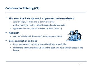
 The most prominent approach to generate recommendations
– used by large, commercial e-commerce sites
– well-understood, various algorithms and variations exist
– applicable in many domains (book, movies, DVDs, ..)
 Approach
– use the "wisdom of the crowd" to recommend items
 Basic assumption and idea
– Users give ratings to catalog items (implicitly or explicitly)
– Customers who had similar tastes in the past, will have similar tastes in the
future
- 4 -
Pure CF Approaches
 Input
– Only a matrix of given user–item ratings
 Output types
– A (numerical) prediction indicating to what degree the current user will like or
dislike a certain item
– A top-N list of recommended items
- 5 -
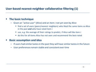
User-based nearest-neighbor collaborative filtering (1)
- 6 -
User-based nearest-neighbor collaborative filtering (2)
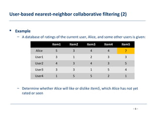
 Example
– A database of ratings of the current user, Alice, and some other users is given:
– Determine whether Alice will like or dislike Item5, which Alice has not yet
rated or seen
Item1 Item2 Item3 Item4 Item5
Alice 5 3 4 4 ?
User1 3 1 2 3 3
User2 4 3 4 3 5
User3 3 3 1 5 4
User4 1 5 5 2 1
- 7 -
User-based nearest-neighbor collaborative filtering (3)
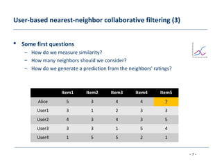
 Some first questions
– How do we measure similarity?
– How many neighbors should we consider?
– How do we generate a prediction from the neighbors' ratings?
Item1 Item2 Item3 Item4 Item5
Alice 5 3 4 4 ?
User1 3 1 2 3 3
User2 4 3 4 3 5
User3 3 3 1 5 4
User4 1 5 5 2 1
- 8 -
Measuring user similarity (1)
- 9 -
Measuring user similarity (2)
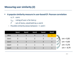
Item1 Item2 Item3 Item4 Item5
Alice 5 3 4 4 ?
User1 3 1 2 3 3
User2 4 3 4 3 5
User3 3 3 1 5 4
User4 1 5 5 2 1
sim = 0,85
sim = 0,00
sim = 0,70
sim = -0,79
- 10 -
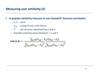
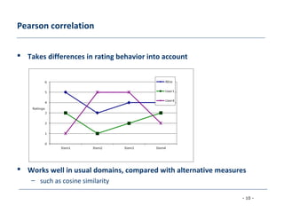
Pearson correlation
 Takes differences in rating behavior into account
 Works well in usual domains, compared with alternative measures
– such as cosine similarity
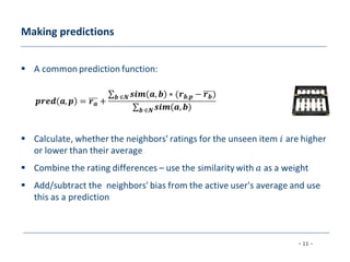
- 11 -
Making predictions
- 12 -
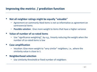
Improving the metrics / prediction function
 Not all neighbor ratings might be equally "valuable"
– Agreement on commonly liked items is not so informative as agreement on
controversial items
– Possible solution: Give more weight to items that have a higher variance
 Value of number of co-rated items
– Use "significance weighting", by e.g., linearly reducing the weight when the
number of co-rated items is low
 Case amplification
– Intuition: Give more weight to "very similar" neighbors, i.e., where the
similarity value is close to 1.
 Neighborhood selection
– Use similarity threshold or fixed number of neighbors
- 13 -
Memory-based and model-based approaches
 User-based CF is said to be "memory-based"
– the rating matrix is directly used to find neighbors / make predictions
– does not scale for most real-world scenarios
– large e-commerce sites have tens of millions of customers and millions of
items
 Model-based approaches
– based on an offline pre-processing or "model-learning" phase
– at run-time, only the learned model is used to make predictions
– models are updated / re-trained periodically
– large variety of techniques used
– model-building and updating can be computationally expensive
– item-based CF is an example for model-based approaches
- 14 -
Item-based collaborative filtering
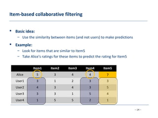
 Basic idea:
– Use the similarity between items (and not users) to make predictions
 Example:
– Look for items that are similar to Item5
– Take Alice's ratings for these items to predict the rating for Item5
Item1 Item2 Item3 Item4 Item5
Alice 5 3 4 4 ?
User1 3 1 2 3 3
User2 4 3 4 3 5
User3 3 3 1 5 4
User4 1 5 5 2 1
- 15 -
The cosine similarity measure
- 16 -
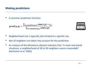
Making predictions
 A common prediction function:
 Neighborhood size is typically also limited to a specific size
 Not all neighbors are taken into account for the prediction
 An analysis of the MovieLens dataset indicates that "in most real-world
situations, a neighborhood of 20 to 50 neighbors seems reasonable"
(Herlocker et al. 2002)
- 17 -
Pre-processing for item-based filtering
 Item-based filtering does not solve the scalability problem itself
 Pre-processing approach by Amazon.com (in 2003)
– Calculate all pair-wise item similarities in advance
– The neighborhood to be used at run-time is typically rather small, because
only items are taken into account which the user has rated
– Item similarities are supposed to be more stable than user similarities
 Memory requirements
– Up to N2
pair-wise similarities to be memorized (N = number of items) in
theory
– In practice, this is significantly lower (items with no co-ratings)
– Further reductions possible
 Minimum threshold for co-ratings
 Limit the neighborhood size (might affect recommendation accuracy)
- 18 -
More on ratings – Explicit ratings
 Probably the most precise ratings
 Most commonly used (1 to 5, 1 to 7 Likert response scales)
 Research topics
– Optimal granularity of scale; indication that 10-point scale is better accepted in movie dom.
– An even more fine-grained scale was chosen in the joke recommender discussed by
Goldberg et al. (2001), where a continuous scale (from −10 to +10) and a graphical input bar
were used
 No precision loss from the discretization
 User preferences can be captured at a finer granularity
 Users actually "like" the graphical interaction method
– Multidimensional ratings (multiple ratings per movie such as ratings for actors and sound)
 Main problems
– Users not always willing to rate many items
 number of available ratings could be too small → sparse rating matrices → poor recommendation
quality
– How to stimulate users to rate more items?
- 19 -
More on ratings – Implicit ratings
 Typically collected by the web shop or application in which the recommender system
is embedded
 When a customer buys an item, for instance, many recommender systems interpret
this behavior as a positive rating
 Clicks, page views, time spent on some page, demo downloads …
 Implicit ratings can be collected constantly and do not require additional efforts from
the side of the user
 Main problem
– One cannot be sure whether the user behavior is correctly interpreted
– For example, a user might not like all the books he or she has bought; the user also might
have bought a book for someone else
 Implicit ratings can be used in addition to explicit ones; question of correctness of
interpretation
- 20 -
Data sparsity problems
 Cold start problem
– How to recommend new items? What to recommend to new users?
 Straightforward approaches
– Ask/force users to rate a set of items
– Use another method (e.g., content-based, demographic or simply non-
personalized) in the initial phase
– Default voting: assign default values to items that only one of the two users to
be compared has rated (Breese et al. 1998)
 Alternatives
– Use better algorithms (beyond nearest-neighbor approaches)
– Example:
 In nearest-neighbor approaches, the set of sufficiently similar neighbors might
be too small to make good predictions
 Assume "transitivity" of neighborhoods
- 21 -
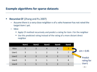
Example algorithms for sparse datasets
Item1 Item2 Item3 Item4 Item5
Alice 5 3 4 4 ?
User1 3 1 2 3 ?
User2 4 3 4 3 5
User3 3 3 1 5 4
User4 1 5 5 2 1
sim = 0.85
Predict
rating for
User1
- 22 -
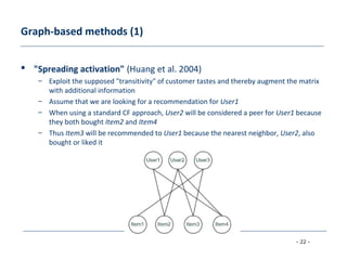
Graph-based methods (1)
 "Spreading activation" (Huang et al. 2004)
– Exploit the supposed "transitivity" of customer tastes and thereby augment the matrix
with additional information
– Assume that we are looking for a recommendation for User1
– When using a standard CF approach, User2 will be considered a peer for User1 because
they both bought Item2 and Item4
– Thus Item3 will be recommended to User1 because the nearest neighbor, User2, also
bought or liked it
- 23 -
Graph-based methods (2)
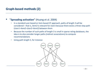
 "Spreading activation" (Huang et al. 2004)
– In a standard user-based or item-based CF approach, paths of length 3 will be
considered – that is, Item3 is relevant for User1 because there exists a three-step path
(User1–Item2–User2–Item3) between them
– Because the number of such paths of length 3 is small in sparse rating databases, the
idea is to also consider longer paths (indirect associations) to compute
recommendations
– Using path length 5, for instance
- 24 -
Graph-based methods (3)
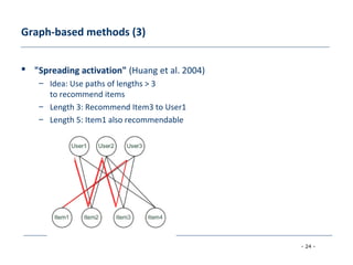
 "Spreading activation" (Huang et al. 2004)
– Idea: Use paths of lengths > 3
to recommend items
– Length 3: Recommend Item3 to User1
– Length 5: Item1 also recommendable
- 25 -
More model-based approaches
 Plethora of different techniques proposed in the last years, e.g.,
– Matrix factorization techniques, statistics
 singular value decomposition, principal component analysis
– Association rule mining
 compare: shopping basket analysis
– Probabilistic models
 clustering models, Bayesian networks, probabilistic Latent Semantic Analysis
– Various other machine learning approaches
 Costs of pre-processing
– Usually not discussed
– Incremental updates possible?
- 26 -
2000: Application of Dimensionality Reduction in
Recommender System, B. Sarwar et al., WebKDD Workshop
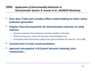
 Basic idea: Trade more complex offline model building for faster online
prediction generation
 Singular Value Decomposition for dimensionality reduction of rating
matrices
– Captures important factors/aspects and their weights in the data
– factors can be genre, actors but also non-understandable ones
– Assumption that k dimensions capture the signals and filter out noise (K = 20 to 100)
 Constant time to make recommendations
 Approach also popular in IR (Latent Semantic Indexing), data
compression,…
- 27 -
Matrix factorization
T
VUM ×Σ×=
- 28 -
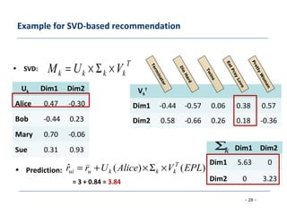
Example for SVD-based recommendation
Vk
T
Dim1 -0.44 -0.57 0.06 0.38 0.57
Dim2 0.58 -0.66 0.26 0.18 -0.36
Uk Dim1 Dim2
Alice 0.47 -0.30
Bob -0.44 0.23
Mary 0.70 -0.06
Sue 0.31 0.93 Dim1 Dim2
Dim1 5.63 0
Dim2 0 3.23
T
kkkk VUM ×Σ×=
kΣ
• SVD:
• Prediction:
= 3 + 0.84 = 3.84
)()(ˆ EPLVAliceUrr T
kkkuui ×Σ×+=
Term
inator
Die
Hard
Twins
EatPray
Love
Pretty
W
om
an
- 29 -
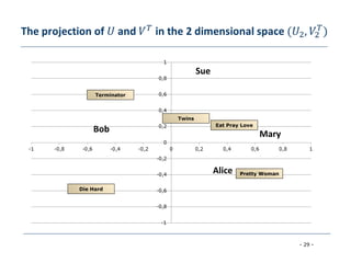
Bob
Mary
Alice
Sue
Eat Pray Love
Pretty Woman
Twins
Die Hard
Terminator
- 30 -
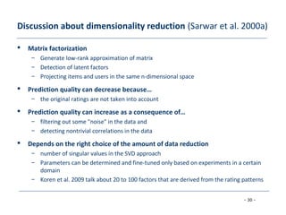
Discussion about dimensionality reduction (Sarwar et al. 2000a)
 Matrix factorization
– Generate low-rank approximation of matrix
– Detection of latent factors
– Projecting items and users in the same n-dimensional space
 Prediction quality can decrease because…
– the original ratings are not taken into account
 Prediction quality can increase as a consequence of…
– filtering out some "noise" in the data and
– detecting nontrivial correlations in the data
 Depends on the right choice of the amount of data reduction
– number of singular values in the SVD approach
– Parameters can be determined and fine-tuned only based on experiments in a certain
domain
– Koren et al. 2009 talk about 20 to 100 factors that are derived from the rating patterns
- 31 -
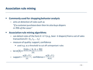
Association rule mining
- 32 -
Recommendation based on Association Rule Mining
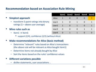
 Simplest approach
– transform 5-point ratings into binary
ratings (1 = above user average)
 Mine rules such as
– Item1 → Item5
 support (2/4), confidence (2/2) (without Alice)
 Make recommendations for Alice (basic method)
– Determine "relevant" rules based on Alice's transactions
(the above rule will be relevant as Alice bought Item1)
– Determine items not already bought by Alice
– Sort the items based on the rules' confidence values
 Different variations possible
– dislike statements, user associations ..
Item1 Item2 Item3 Item4 Item5
Alice 1 0 0 0 ?
User1 1 0 1 0 1
User2 1 0 1 0 1
User3 0 0 0 1 1
User4 0 1 1 0 0
- 33 -
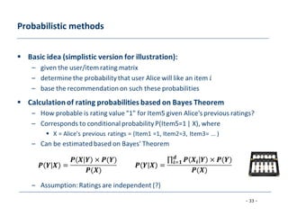
Probabilistic methods
- 34 -
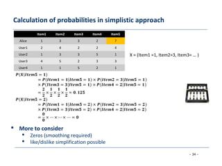
Calculation of probabilities in simplistic approach
Item1 Item2 Item3 Item4 Item5
Alice 1 3 3 2 ?
User1 2 4 2 2 4
User2 1 3 3 5 1
User3 4 5 2 3 3
User4 1 1 5 2 1
 More to consider
 Zeros (smoothing required)
 like/dislike simplification possible
X = (Item1 =1, Item2=3, Item3= … )
- 35 -
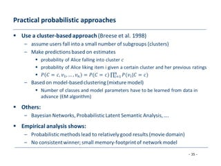
Practical probabilistic approaches
- 36 -
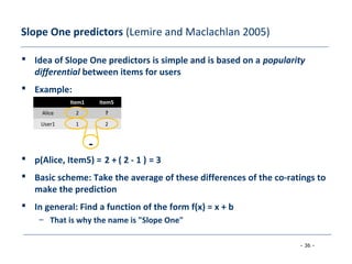
Item1 Item5
Alice 2 ?
User1 1 2
 Idea of Slope One predictors is simple and is based on a popularity
differential between items for users
 Example:
 p(Alice, Item5) =
 Basic scheme: Take the average of these differences of the co-ratings to
make the prediction
 In general: Find a function of the form f(x) = x + b
– That is why the name is "Slope One"
Slope One predictors (Lemire and Maclachlan 2005)
-
2 + ( 2 - 1 ) = 3
- 37 -
RF-Rec predictors (Gedikli et al. 2011)
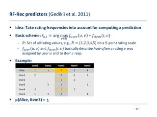
Item1 Item2 Item3 Item4 Item5
Alice 1 1 ? 5 4
User1 2 5 5 5
User2 1 1
User3 5 2 2
User4 3 1 1
User5 1 2 2 4
1
- 38 -
2008: Factorization meets the neighborhood: a multifaceted
collaborative
filtering model, Y. Koren, ACM SIGKDD
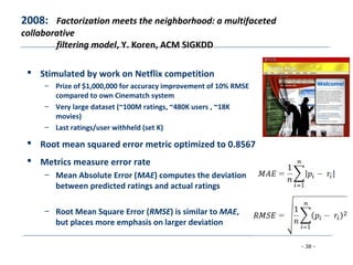
 Stimulated by work on Netflix competition
– Prize of $1,000,000 for accuracy improvement of 10% RMSE
compared to own Cinematch system
– Very large dataset (~100M ratings, ~480K users , ~18K
movies)
– Last ratings/user withheld (set K)
 Root mean squared error metric optimized to 0.8567
 Metrics measure error rate
– Mean Absolute Error (MAE) computes the deviation
between predicted ratings and actual ratings
– Root Mean Square Error (RMSE) is similar to MAE,
but places more emphasis on larger deviation
- 39 -
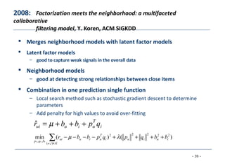
 Merges neighborhood models with latent factor models
 Latent factor models
– good to capture weak signals in the overall data
 Neighborhood models
– good at detecting strong relationships between close items
 Combination in one prediction single function
– Local search method such as stochastic gradient descent to determine
parameters
– Add penalty for high values to avoid over-fitting
2008: Factorization meets the neighborhood: a multifaceted
collaborative
filtering model, Y. Koren, ACM SIGKDD
∑∈
++++−−−−
Kiu
iuiui
T
uiuui
bqp
bbqpqpbbr
),(
22222
,,
)()(min
***
λµ
i
T
uiuui qpbbr +++= µˆ
- 40 -
Summarizing recent methods
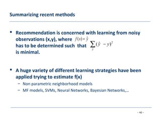
 Recommendation is concerned with learning from noisy
observations (x,y), where
has to be determined such that
is minimal.
 A huge variety of different learning strategies have been
applied trying to estimate f(x)
– Non parametric neighborhood models
– MF models, SVMs, Neural Networks, Bayesian Networks,…
yxf ˆ)( =
∑ −
y
yy
ˆ
2
)ˆ(
- 41 -
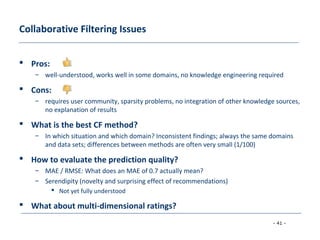
Collaborative Filtering Issues
 Pros:
– well-understood, works well in some domains, no knowledge engineering required
 Cons:
– requires user community, sparsity problems, no integration of other knowledge sources,
no explanation of results
 What is the best CF method?
– In which situation and which domain? Inconsistent findings; always the same domains
and data sets; differences between methods are often very small (1/100)
 How to evaluate the prediction quality?
– MAE / RMSE: What does an MAE of 0.7 actually mean?
– Serendipity (novelty and surprising effect of recommendations)
 Not yet fully understood
 What about multi-dimensional ratings?
- 42 -
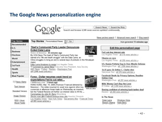
The Google News personalization engine
- 43 -
Google News portal (1)
 Aggregates news articles from several thousand sources
 Displays them to signed-in users in a personalized way
 Collaborative recommendation approach based on
– the click history of the active user and
– the history of the larger community
 Main challenges
– Vast number of articles and users
– Generate recommendation list in real time (at most one second)
– Constant stream of new items
– Immediately react to user interaction
 Significant efforts with respect to algorithms, engineering, and
parallelization are required
- 44 -
Google News portal (2)
 Pure memory-based approaches are not directly applicable and for
model-based approaches, the problem of continuous model updates
must be solved
 A combination of model- and memory-based techniques is used
 Model-based part: Two clustering techniques are used
– Probabilistic Latent Semantic Indexing (PLSI) as proposed by (Hofmann 2004)
– MinHash as a hashing method
 Memory-based part: Analyze story co-visits for dealing with new users
 Google's MapReduce technique is used for parallelization in order to
make computation scalable
- 45 -
Literature (1)
 [Adomavicius and Tuzhilin 2005] Toward the next generation of recommender systems: A survey of the state-of-the-art
and possible extensions, IEEE Transactions on Knowledge and Data Engineering 17 (2005), no. 6, 734–749
 [Breese et al. 1998] Empirical analysis of predictive algorithms for collaborative filtering, Proceedings of the 14th
Conference on Uncertainty in Artificial Intelligence (Madison, WI) (Gregory F. Cooper and Seraf´in Moral, eds.), Morgan
Kaufmann, 1998, pp. 43–52
 [Gedikli et al. 2011] RF-Rec: Fast and accurate computation of recommendations based on rating frequencies, Proceedings
of the 13th IEEE Conference on Commerce and Enterprise Computing - CEC 2011, Luxembourg, 2011, forthcoming
 [Goldberg et al. 2001] Eigentaste: A constant time collaborative filtering algorithm, Information Retrieval 4 (2001), no. 2,
133–151
 [Golub and Kahan 1965] Calculating the singular values and pseudo-inverse of a matrix, Journal of the Society for Industrial
and Applied Mathematics, Series B: Numerical Analysis 2 (1965), no. 2, 205–224
 [Herlocker et al. 2002] An empirical analysis of design choices in neighborhood-based collaborative filtering algorithms,
Information Retrieval 5 (2002), no. 4, 287–310
 [Herlocker et al. 2004] Evaluating collaborative filtering recommender systems, ACM Transactions on Information Systems
(TOIS) 22 (2004), no. 1, 5–53
- 46 -
Literature (2)
 [Hofmann 2004] Latent semantic models for collaborative filtering, ACM Transactions on Information Systems 22 (2004),
no. 1, 89–115
 [Huang et al. 2004] Applying associative retrieval techniques to alleviate the sparsity problem in collaborative filtering,
ACM Transactions on Information Systems 22 (2004), no. 1, 116–142
 [Koren et al. 2009] Matrix factorization techniques for recommender systems, Computer 42 (2009), no. 8, 30–37
 [Lemire and Maclachlan 2005] Slope one predictors for online rating-based collaborative filtering, Proceedings of the 5th
SIAM International Conference on Data Mining (SDM ’05) (Newport Beach, CA), 2005, pp. 471–480
 [Sarwar et al. 2000a] Application of dimensionality reduction in recommender systems – a case study, Proceedings of the
ACM WebKDD Workshop (Boston), 2000
 [Zhang and Pu 2007] A recursive prediction algorithm for collaborative filtering recommender systems, Proceedings of the
2007 ACM Conference on Recommender Systems (RecSys ’07) (Minneapolis, MN), ACM, 2007, pp. 57–64

Chapter 02 collaborative recommendation

  • 1.
  • 2.
    - 2 - Agenda Collaborative Filtering (CF) – Pure CF approaches – User-based nearest-neighbor – The Pearson Correlation similarity measure – Memory-based and model-based approaches – Item-based nearest-neighbor – The cosine similarity measure – Data sparsity problems – Recent methods (SVD, Association Rule Mining, Slope One, RF-Rec, …) – The Google News personalization engine – Discussion and summary – Literature
  • 3.
    - 3 - CollaborativeFiltering (CF)  The most prominent approach to generate recommendations – used by large, commercial e-commerce sites – well-understood, various algorithms and variations exist – applicable in many domains (book, movies, DVDs, ..)  Approach – use the "wisdom of the crowd" to recommend items  Basic assumption and idea – Users give ratings to catalog items (implicitly or explicitly) – Customers who had similar tastes in the past, will have similar tastes in the future
  • 4.
    - 4 - PureCF Approaches  Input – Only a matrix of given user–item ratings  Output types – A (numerical) prediction indicating to what degree the current user will like or dislike a certain item – A top-N list of recommended items
  • 5.
    - 5 - User-basednearest-neighbor collaborative filtering (1)
  • 6.
    - 6 - User-basednearest-neighbor collaborative filtering (2)  Example – A database of ratings of the current user, Alice, and some other users is given: – Determine whether Alice will like or dislike Item5, which Alice has not yet rated or seen Item1 Item2 Item3 Item4 Item5 Alice 5 3 4 4 ? User1 3 1 2 3 3 User2 4 3 4 3 5 User3 3 3 1 5 4 User4 1 5 5 2 1
  • 7.
    - 7 - User-basednearest-neighbor collaborative filtering (3)  Some first questions – How do we measure similarity? – How many neighbors should we consider? – How do we generate a prediction from the neighbors' ratings? Item1 Item2 Item3 Item4 Item5 Alice 5 3 4 4 ? User1 3 1 2 3 3 User2 4 3 4 3 5 User3 3 3 1 5 4 User4 1 5 5 2 1
  • 8.
    - 8 - Measuringuser similarity (1)
  • 9.
    - 9 - Measuringuser similarity (2) Item1 Item2 Item3 Item4 Item5 Alice 5 3 4 4 ? User1 3 1 2 3 3 User2 4 3 4 3 5 User3 3 3 1 5 4 User4 1 5 5 2 1 sim = 0,85 sim = 0,00 sim = 0,70 sim = -0,79
  • 10.
    - 10 - Pearsoncorrelation  Takes differences in rating behavior into account  Works well in usual domains, compared with alternative measures – such as cosine similarity
  • 11.
    - 11 - Makingpredictions
  • 12.
    - 12 - Improvingthe metrics / prediction function  Not all neighbor ratings might be equally "valuable" – Agreement on commonly liked items is not so informative as agreement on controversial items – Possible solution: Give more weight to items that have a higher variance  Value of number of co-rated items – Use "significance weighting", by e.g., linearly reducing the weight when the number of co-rated items is low  Case amplification – Intuition: Give more weight to "very similar" neighbors, i.e., where the similarity value is close to 1.  Neighborhood selection – Use similarity threshold or fixed number of neighbors
  • 13.
    - 13 - Memory-basedand model-based approaches  User-based CF is said to be "memory-based" – the rating matrix is directly used to find neighbors / make predictions – does not scale for most real-world scenarios – large e-commerce sites have tens of millions of customers and millions of items  Model-based approaches – based on an offline pre-processing or "model-learning" phase – at run-time, only the learned model is used to make predictions – models are updated / re-trained periodically – large variety of techniques used – model-building and updating can be computationally expensive – item-based CF is an example for model-based approaches
  • 14.
    - 14 - Item-basedcollaborative filtering  Basic idea: – Use the similarity between items (and not users) to make predictions  Example: – Look for items that are similar to Item5 – Take Alice's ratings for these items to predict the rating for Item5 Item1 Item2 Item3 Item4 Item5 Alice 5 3 4 4 ? User1 3 1 2 3 3 User2 4 3 4 3 5 User3 3 3 1 5 4 User4 1 5 5 2 1
  • 15.
    - 15 - Thecosine similarity measure
  • 16.
    - 16 - Makingpredictions  A common prediction function:  Neighborhood size is typically also limited to a specific size  Not all neighbors are taken into account for the prediction  An analysis of the MovieLens dataset indicates that "in most real-world situations, a neighborhood of 20 to 50 neighbors seems reasonable" (Herlocker et al. 2002)
  • 17.
    - 17 - Pre-processingfor item-based filtering  Item-based filtering does not solve the scalability problem itself  Pre-processing approach by Amazon.com (in 2003) – Calculate all pair-wise item similarities in advance – The neighborhood to be used at run-time is typically rather small, because only items are taken into account which the user has rated – Item similarities are supposed to be more stable than user similarities  Memory requirements – Up to N2 pair-wise similarities to be memorized (N = number of items) in theory – In practice, this is significantly lower (items with no co-ratings) – Further reductions possible  Minimum threshold for co-ratings  Limit the neighborhood size (might affect recommendation accuracy)
  • 18.
    - 18 - Moreon ratings – Explicit ratings  Probably the most precise ratings  Most commonly used (1 to 5, 1 to 7 Likert response scales)  Research topics – Optimal granularity of scale; indication that 10-point scale is better accepted in movie dom. – An even more fine-grained scale was chosen in the joke recommender discussed by Goldberg et al. (2001), where a continuous scale (from −10 to +10) and a graphical input bar were used  No precision loss from the discretization  User preferences can be captured at a finer granularity  Users actually "like" the graphical interaction method – Multidimensional ratings (multiple ratings per movie such as ratings for actors and sound)  Main problems – Users not always willing to rate many items  number of available ratings could be too small → sparse rating matrices → poor recommendation quality – How to stimulate users to rate more items?
  • 19.
    - 19 - Moreon ratings – Implicit ratings  Typically collected by the web shop or application in which the recommender system is embedded  When a customer buys an item, for instance, many recommender systems interpret this behavior as a positive rating  Clicks, page views, time spent on some page, demo downloads …  Implicit ratings can be collected constantly and do not require additional efforts from the side of the user  Main problem – One cannot be sure whether the user behavior is correctly interpreted – For example, a user might not like all the books he or she has bought; the user also might have bought a book for someone else  Implicit ratings can be used in addition to explicit ones; question of correctness of interpretation
  • 20.
    - 20 - Datasparsity problems  Cold start problem – How to recommend new items? What to recommend to new users?  Straightforward approaches – Ask/force users to rate a set of items – Use another method (e.g., content-based, demographic or simply non- personalized) in the initial phase – Default voting: assign default values to items that only one of the two users to be compared has rated (Breese et al. 1998)  Alternatives – Use better algorithms (beyond nearest-neighbor approaches) – Example:  In nearest-neighbor approaches, the set of sufficiently similar neighbors might be too small to make good predictions  Assume "transitivity" of neighborhoods
  • 21.
    - 21 - Examplealgorithms for sparse datasets Item1 Item2 Item3 Item4 Item5 Alice 5 3 4 4 ? User1 3 1 2 3 ? User2 4 3 4 3 5 User3 3 3 1 5 4 User4 1 5 5 2 1 sim = 0.85 Predict rating for User1
  • 22.
    - 22 - Graph-basedmethods (1)  "Spreading activation" (Huang et al. 2004) – Exploit the supposed "transitivity" of customer tastes and thereby augment the matrix with additional information – Assume that we are looking for a recommendation for User1 – When using a standard CF approach, User2 will be considered a peer for User1 because they both bought Item2 and Item4 – Thus Item3 will be recommended to User1 because the nearest neighbor, User2, also bought or liked it
  • 23.
    - 23 - Graph-basedmethods (2)  "Spreading activation" (Huang et al. 2004) – In a standard user-based or item-based CF approach, paths of length 3 will be considered – that is, Item3 is relevant for User1 because there exists a three-step path (User1–Item2–User2–Item3) between them – Because the number of such paths of length 3 is small in sparse rating databases, the idea is to also consider longer paths (indirect associations) to compute recommendations – Using path length 5, for instance
  • 24.
    - 24 - Graph-basedmethods (3)  "Spreading activation" (Huang et al. 2004) – Idea: Use paths of lengths > 3 to recommend items – Length 3: Recommend Item3 to User1 – Length 5: Item1 also recommendable
  • 25.
    - 25 - Moremodel-based approaches  Plethora of different techniques proposed in the last years, e.g., – Matrix factorization techniques, statistics  singular value decomposition, principal component analysis – Association rule mining  compare: shopping basket analysis – Probabilistic models  clustering models, Bayesian networks, probabilistic Latent Semantic Analysis – Various other machine learning approaches  Costs of pre-processing – Usually not discussed – Incremental updates possible?
  • 26.
    - 26 - 2000:Application of Dimensionality Reduction in Recommender System, B. Sarwar et al., WebKDD Workshop  Basic idea: Trade more complex offline model building for faster online prediction generation  Singular Value Decomposition for dimensionality reduction of rating matrices – Captures important factors/aspects and their weights in the data – factors can be genre, actors but also non-understandable ones – Assumption that k dimensions capture the signals and filter out noise (K = 20 to 100)  Constant time to make recommendations  Approach also popular in IR (Latent Semantic Indexing), data compression,…
  • 27.
    - 27 - Matrixfactorization T VUM ×Σ×=
  • 28.
    - 28 - Examplefor SVD-based recommendation Vk T Dim1 -0.44 -0.57 0.06 0.38 0.57 Dim2 0.58 -0.66 0.26 0.18 -0.36 Uk Dim1 Dim2 Alice 0.47 -0.30 Bob -0.44 0.23 Mary 0.70 -0.06 Sue 0.31 0.93 Dim1 Dim2 Dim1 5.63 0 Dim2 0 3.23 T kkkk VUM ×Σ×= kΣ • SVD: • Prediction: = 3 + 0.84 = 3.84 )()(ˆ EPLVAliceUrr T kkkuui ×Σ×+= Term inator Die Hard Twins EatPray Love Pretty W om an
  • 29.
    - 29 - Bob Mary Alice Sue EatPray Love Pretty Woman Twins Die Hard Terminator
  • 30.
    - 30 - Discussionabout dimensionality reduction (Sarwar et al. 2000a)  Matrix factorization – Generate low-rank approximation of matrix – Detection of latent factors – Projecting items and users in the same n-dimensional space  Prediction quality can decrease because… – the original ratings are not taken into account  Prediction quality can increase as a consequence of… – filtering out some "noise" in the data and – detecting nontrivial correlations in the data  Depends on the right choice of the amount of data reduction – number of singular values in the SVD approach – Parameters can be determined and fine-tuned only based on experiments in a certain domain – Koren et al. 2009 talk about 20 to 100 factors that are derived from the rating patterns
  • 31.
    - 31 - Associationrule mining
  • 32.
    - 32 - Recommendationbased on Association Rule Mining  Simplest approach – transform 5-point ratings into binary ratings (1 = above user average)  Mine rules such as – Item1 → Item5  support (2/4), confidence (2/2) (without Alice)  Make recommendations for Alice (basic method) – Determine "relevant" rules based on Alice's transactions (the above rule will be relevant as Alice bought Item1) – Determine items not already bought by Alice – Sort the items based on the rules' confidence values  Different variations possible – dislike statements, user associations .. Item1 Item2 Item3 Item4 Item5 Alice 1 0 0 0 ? User1 1 0 1 0 1 User2 1 0 1 0 1 User3 0 0 0 1 1 User4 0 1 1 0 0
  • 33.
  • 34.
    - 34 - Calculationof probabilities in simplistic approach Item1 Item2 Item3 Item4 Item5 Alice 1 3 3 2 ? User1 2 4 2 2 4 User2 1 3 3 5 1 User3 4 5 2 3 3 User4 1 1 5 2 1  More to consider  Zeros (smoothing required)  like/dislike simplification possible X = (Item1 =1, Item2=3, Item3= … )
  • 35.
    - 35 - Practicalprobabilistic approaches
  • 36.
    - 36 - Item1Item5 Alice 2 ? User1 1 2  Idea of Slope One predictors is simple and is based on a popularity differential between items for users  Example:  p(Alice, Item5) =  Basic scheme: Take the average of these differences of the co-ratings to make the prediction  In general: Find a function of the form f(x) = x + b – That is why the name is "Slope One" Slope One predictors (Lemire and Maclachlan 2005) - 2 + ( 2 - 1 ) = 3
  • 37.
    - 37 - RF-Recpredictors (Gedikli et al. 2011) Item1 Item2 Item3 Item4 Item5 Alice 1 1 ? 5 4 User1 2 5 5 5 User2 1 1 User3 5 2 2 User4 3 1 1 User5 1 2 2 4 1
  • 38.
    - 38 - 2008:Factorization meets the neighborhood: a multifaceted collaborative filtering model, Y. Koren, ACM SIGKDD  Stimulated by work on Netflix competition – Prize of $1,000,000 for accuracy improvement of 10% RMSE compared to own Cinematch system – Very large dataset (~100M ratings, ~480K users , ~18K movies) – Last ratings/user withheld (set K)  Root mean squared error metric optimized to 0.8567  Metrics measure error rate – Mean Absolute Error (MAE) computes the deviation between predicted ratings and actual ratings – Root Mean Square Error (RMSE) is similar to MAE, but places more emphasis on larger deviation
  • 39.
    - 39 - Merges neighborhood models with latent factor models  Latent factor models – good to capture weak signals in the overall data  Neighborhood models – good at detecting strong relationships between close items  Combination in one prediction single function – Local search method such as stochastic gradient descent to determine parameters – Add penalty for high values to avoid over-fitting 2008: Factorization meets the neighborhood: a multifaceted collaborative filtering model, Y. Koren, ACM SIGKDD ∑∈ ++++−−−− Kiu iuiui T uiuui bqp bbqpqpbbr ),( 22222 ,, )()(min *** λµ i T uiuui qpbbr +++= µˆ
  • 40.
    - 40 - Summarizingrecent methods  Recommendation is concerned with learning from noisy observations (x,y), where has to be determined such that is minimal.  A huge variety of different learning strategies have been applied trying to estimate f(x) – Non parametric neighborhood models – MF models, SVMs, Neural Networks, Bayesian Networks,… yxf ˆ)( = ∑ − y yy ˆ 2 )ˆ(
  • 41.
    - 41 - CollaborativeFiltering Issues  Pros: – well-understood, works well in some domains, no knowledge engineering required  Cons: – requires user community, sparsity problems, no integration of other knowledge sources, no explanation of results  What is the best CF method? – In which situation and which domain? Inconsistent findings; always the same domains and data sets; differences between methods are often very small (1/100)  How to evaluate the prediction quality? – MAE / RMSE: What does an MAE of 0.7 actually mean? – Serendipity (novelty and surprising effect of recommendations)  Not yet fully understood  What about multi-dimensional ratings?
  • 42.
    - 42 - TheGoogle News personalization engine
  • 43.
    - 43 - GoogleNews portal (1)  Aggregates news articles from several thousand sources  Displays them to signed-in users in a personalized way  Collaborative recommendation approach based on – the click history of the active user and – the history of the larger community  Main challenges – Vast number of articles and users – Generate recommendation list in real time (at most one second) – Constant stream of new items – Immediately react to user interaction  Significant efforts with respect to algorithms, engineering, and parallelization are required
  • 44.
    - 44 - GoogleNews portal (2)  Pure memory-based approaches are not directly applicable and for model-based approaches, the problem of continuous model updates must be solved  A combination of model- and memory-based techniques is used  Model-based part: Two clustering techniques are used – Probabilistic Latent Semantic Indexing (PLSI) as proposed by (Hofmann 2004) – MinHash as a hashing method  Memory-based part: Analyze story co-visits for dealing with new users  Google's MapReduce technique is used for parallelization in order to make computation scalable
  • 45.
    - 45 - Literature(1)  [Adomavicius and Tuzhilin 2005] Toward the next generation of recommender systems: A survey of the state-of-the-art and possible extensions, IEEE Transactions on Knowledge and Data Engineering 17 (2005), no. 6, 734–749  [Breese et al. 1998] Empirical analysis of predictive algorithms for collaborative filtering, Proceedings of the 14th Conference on Uncertainty in Artificial Intelligence (Madison, WI) (Gregory F. Cooper and Seraf´in Moral, eds.), Morgan Kaufmann, 1998, pp. 43–52  [Gedikli et al. 2011] RF-Rec: Fast and accurate computation of recommendations based on rating frequencies, Proceedings of the 13th IEEE Conference on Commerce and Enterprise Computing - CEC 2011, Luxembourg, 2011, forthcoming  [Goldberg et al. 2001] Eigentaste: A constant time collaborative filtering algorithm, Information Retrieval 4 (2001), no. 2, 133–151  [Golub and Kahan 1965] Calculating the singular values and pseudo-inverse of a matrix, Journal of the Society for Industrial and Applied Mathematics, Series B: Numerical Analysis 2 (1965), no. 2, 205–224  [Herlocker et al. 2002] An empirical analysis of design choices in neighborhood-based collaborative filtering algorithms, Information Retrieval 5 (2002), no. 4, 287–310  [Herlocker et al. 2004] Evaluating collaborative filtering recommender systems, ACM Transactions on Information Systems (TOIS) 22 (2004), no. 1, 5–53
  • 46.
    - 46 - Literature(2)  [Hofmann 2004] Latent semantic models for collaborative filtering, ACM Transactions on Information Systems 22 (2004), no. 1, 89–115  [Huang et al. 2004] Applying associative retrieval techniques to alleviate the sparsity problem in collaborative filtering, ACM Transactions on Information Systems 22 (2004), no. 1, 116–142  [Koren et al. 2009] Matrix factorization techniques for recommender systems, Computer 42 (2009), no. 8, 30–37  [Lemire and Maclachlan 2005] Slope one predictors for online rating-based collaborative filtering, Proceedings of the 5th SIAM International Conference on Data Mining (SDM ’05) (Newport Beach, CA), 2005, pp. 471–480  [Sarwar et al. 2000a] Application of dimensionality reduction in recommender systems – a case study, Proceedings of the ACM WebKDD Workshop (Boston), 2000  [Zhang and Pu 2007] A recursive prediction algorithm for collaborative filtering recommender systems, Proceedings of the 2007 ACM Conference on Recommender Systems (RecSys ’07) (Minneapolis, MN), ACM, 2007, pp. 57–64