This document describes the adaptive restore algorithm, a non-reversible Markov chain Monte Carlo method. It begins with an overview of the restore process, which takes regenerations from an underlying diffusion or jump process to construct a reversible Markov chain with a target distribution. The adaptive restore process enriches this by allowing the regeneration distribution to adapt over time. It converges almost surely to the minimal regeneration distribution. Parameters like the initial regeneration distribution and rates are discussed. Examples are provided for the adaptive Brownian restore algorithm and calibrating the parameters.

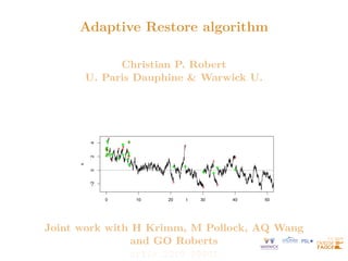
1. Adaptive Restore algorithm
Christian P. Robert
U. Paris Dauphine & Warwick U.
0 10 20 30 40 50
−2
0
2
4
x
t
Joint work with H Krimm, M Pollock, AQ Wang
and GO Roberts
arXiv:2210.09901

2. EaRly Call
Incoming 2023-2030 ERC funding for postdoctoral
collaborations with
I Michael Jordan (Berkeley)
I Eric Moulines (Paris)
I Gareth Roberts (Warwick)
I myself (Paris)

3. MCMC regeneration
Reversibility attached with (sub-efficient) random walk
behaviour
Recent achievements in non-reversible MCMC with PDMPs
[Bouchard-Côté et al., 2018; Bierkens et al., 2019]
Linked with regeneration
[Nummelin, 1978; Mykland et al., X, 1995]

4. Restore process
Take {Yt}t≥0 diffusion / jump process on Rd with infinitesimal
generator LY and Y0 ∼ µ —e..g., LY = ∆/2 for Brownian—
Regeneration rate κ with associated tour length
τ = inf t ≥ 0 :
Zt
0
κ(Ys)ds ≥ ξ ξ ∼ Exp(1)
Take {Y
(i)
t }t≥0, τ(i)
∞
i=0
iid realisations
Regeneration times Tj =
Pj−1
i=0 τ(i)
Restore process {Xt}t≥0 given by:
Xt =
∞
X
i=0
I[Ti,Ti+1)(t)Y
(i)
t−Ti
[Wang et al., 2021]

5. Restore process
0 2 4 6 8
−2
−1
0
1
2
x
t
Path of 5 tours of Brownian Restore with
π ≡ N(0, 12), µ ≡ N(0, 22) and C chosen so that
minx∈R κ(x) = 0, with K = 200 and Λ0 = 1000. First and last
output states shown by green dots and red crosses

6. Stationarity of Restore
Infinitesimal generator of {Xt}t≥0
LXf(x) = LYf(x) + κ(x)
Z
[f(y) − f(x)]µ(y)dy
Regeneration rate κ chosen as1
κ(x) =
L†
Yπ(x)
π(x)
+ C
µ(x)
π(x)
makes {Xt}t≥0 π-invariant
Z
Rd
LXf(x)π(x)dx = 0
1
L†
Y formal adjoint

7. Restore sampler
Rewrite
κ(x) =
L†
Yπ(x)
π(x)
+ C
µ(x)
π(x)
= κ̃(x) + C
µ(x)
π(x)
with
I κ̃ partial regeneration rate
I C 0 regeneration constant and
I Cµ regeneration measure, large enough so that κ(·) 0
Resulting Monte Carlo method called Restore Sampler
[Wang et al., 2021]

8. Restore sampler
Given π-invariance of {Xt}t≥0
Eπ[f] = EX0∼µ
h Zτ(0)
0
f(Xs)dx
i.
EX0∼µ[τ(0)
]
and a.s. convergence of ergodic averages:
1
t
Zt
0
f(Xs)ds → Eπ[f]
For iid Zi :=
RTi+1
Ti
f(Xs)ds, CLT
√
n
ZTn
0
f(Xs)dx
Tn − Eπ[f]
!
→ N(0, σ2
f)
where
σ2
f := EX0∼µ
Z0 − τ(0)
Eπ[f]
2
.
EX0∼µ[τ(0)
]
2

9. Restore sampler
Given π-invariance of {Xt}t≥0
Eπ[f] = EX0∼µ
h Zτ(0)
0
f(Xs)dx
i.
EX0∼µ[τ(0)
]
and a.s. convergence of ergodic averages:
1
t
Zt
0
f(Xs)ds → Eπ[f]
Estimator variance depends on expected tour length: choose µ
towards long tours
[Wang et al., 2020]

10. Minimal regeneration
Minimal regeneration measure, C+µ+ corresponding to smallest
possible rate
κ+
(x) := κ̃(x) ∨ 0 = κ̃(x) + C+ µ+(x)
π(x)
leading to
µ+
(x) =
1
C+
[0 ∨ −κ̃(x)]π(x)
Frequent regeneration not necessarily detrimental, except when
when µ is not well-aligned to π, leading to wasted computation
Minimal Restore maximizes expected tour length / minimizes
asymptotic variance
[Wang et al., 2021]

11. Constant approximation
When target misses normalizing constant
π(x) = π̃(x)
Z,
take energy U(x) := − log π(x) = log Z − log π̃(x)
When {Yt}t≥0 Brownian, κ̃ function of ∇U(x) and ∆U(x)

12. Constant approximation
When target misses normalizing constant
π(x) = π̃(x)
Z,
take energy U(x) := − log π(x) = log Z − log π̃(x)
When {Yt}t≥0 Brownian, κ̃ function of ∇U(x) and ∆U(x)
In regeneration rate, Z “absorbed” into C
κ(x) = κ̃(x) + C
µ(x)
π̃(x)
Z
= κ̃(x) + CZ
µ(x)
π̃(x)
= κ̃(x) + C̃
µ(x)
π̃(x)
,
where C̃ = CZ set by user. Since C = 1/Eµ[τ] Using n tours
with simulation time T, Z ≈ C̃T
n.

13. Adapting Restore
Adaptive Restore process defined by enriching underlying
continuous-time Markov process with regenerations at rate κ+
from distribution µt at time t
Convergence of (µt, πt) to (µ+, π): a.s. convergence of stochastic
approximation algorithms for discrete-time processes on
compact spaces
[Benaı̈m et al., 2018]

14. Adapting Restore
Initial regeneration distribution µ0 and updates by addition of
point masses
µt(x) =
µ0(x), if N(t) = 0,
t
a+t
1
N(t)
PN(t)
i=1 δXζi
(x) + a
a+t µ0(x), if N(t) 0,
where a 0 constant2 and ζi arrival times of inhomogeneous
Poisson process (N(t) : t ≥ 0) with rate κ−(Xt)
κ−
(x) := [0 ∨ −κ̃(x)]
Poisson process simulated by Poisson thinning, under
assumption
K−
:= sup
x∈X
κ−
(x) 0
2
Discrete measure dominance time: when regeneration most likely to be
from discrete measure in mixture distribution

15. Adaptive Brownian Restore Algorithm
t ← 0, E ← ∅, i ← 0, X ∼ µ0.
while i n do
τ̃ ∼ Exp(K+
), s ∼ Exp(Λ0), ζ̃ ∼ Exp(K−
).
if τ̃ s and τ̃ ζ̃ then
X ∼ N(X, τ̃), t ← t + τ̃, u ∼ U[0, 1].
if u κ+
(X)/K+
then
if |E| = 0 then
X ∼ µ0.
else
X ∼ U(E) with probability t/(a + t), else X ∼ µ0.
end
i ← i + 1.
end
else if s τ̃ and s ζ̃ then
X ∼ N(X, s), t ← t + s, record X, t, i.
else
X ∼ N(X, ζ̃), t ← t + ζ̃, u ∼ U[0, 1].
If u κ−
(X)/K−
then E ← E ∪ {X}.
end
end

16. Adaptive Brownian Restore Algorithm
0 10 20 30 40 50
−2
0
2
4
x
t
Path of an Adaptive Brownian Restore process with
π ≡ N(0, 1), µ0 ≡ N(2, 1), a = 10. Green dots and red crosses
show the first and last output states of each tour.

17. Calibrating initial regeneration and parameters
I µ0 as initial approximate π, e.g., µ0 ≡ Nd(0, I) with π
pre-transformed
I Tradeoff in choosing a discrete measure dominance time:
smaller choices of a lead to faster convergence while larger
value of a produces more regenerations from µ0, hence
better exploration (range of a between 1,000 and 10,000)
I K+ and K− based on quantiles of κ̃, from preliminary
MCMC run
I or, assuming π close to Gaussian, initial guess of K− is d/2
and initial estimate for K+ based on chi-squared
approximation

18. Final remarks
I Adaptive Restore benefits from global moves, for targets
hard to approximate with a parametric distribution, with
large moves across the space
I Use of minimal regeneration rate makes simulation
computationally feasible and more likely in areas where π
has significant mass
I In comparison to e.g. Random Walk Metropolis, process
can be slow but higher efficiency in sampling distributions
with skewed tails