Downloaded 827 times
![Navier-Stokes Equations
V ρa = ∑ F
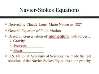
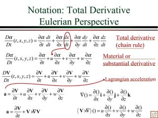
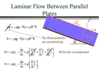
Navier-Stokes Equation
ρ a + ρ g = −∇p + µ∇ V 2
g is constant
ρ a = − ( ∇p + ρ g ) + µ∇ 2 V a is a function of t, x, y, z
ρa = Inertial forces [N/m3], a is Lagrangian acceleration
Is acceleration zero when ∂V/ ∂ t = 0? NO!
− ( ∇p + ρ g ) = Pressure gradient (not due to change in elevation)
∇p + ρ g ≠ 0 V ≠0
If _________ then _____
du
µ∇ V = Shear stress gradient
2 τ =µ τ = µ∇V
dx](https://image.slidesharecdn.com/basicdifferentialequationsinfluidmechanics-121127123302-phpapp01/85/Basic-differential-equations-in-fluid-mechanics-8-320.jpg)


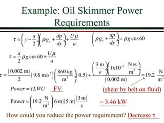
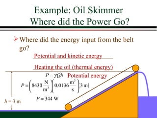
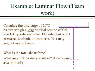
![Example: Oil Skimmer Power
Requirements
How do we get the power requirement?
___________________________
Power = Force x Velocity [N·m/s]
What is the force acting on the belt?
Shear force (τ·L · W)
___________________________
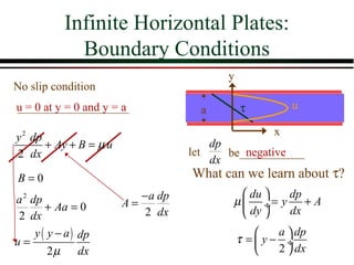
Remember the equation for shear?
τ=µ(du/dy)
_____________ Evaluate at y = a.
du dp Uµ a dp
µ = y ρ g x + ÷+ A A= − ρ gx + ÷
dy dx a 2 dx
a dp U µ
τ = y − ÷ ρ g x + ÷+
2 dx a](https://image.slidesharecdn.com/basicdifferentialequationsinfluidmechanics-121127123302-phpapp01/85/Basic-differential-equations-in-fluid-mechanics-22-320.jpg)
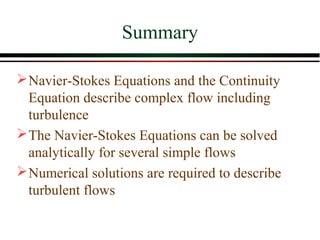

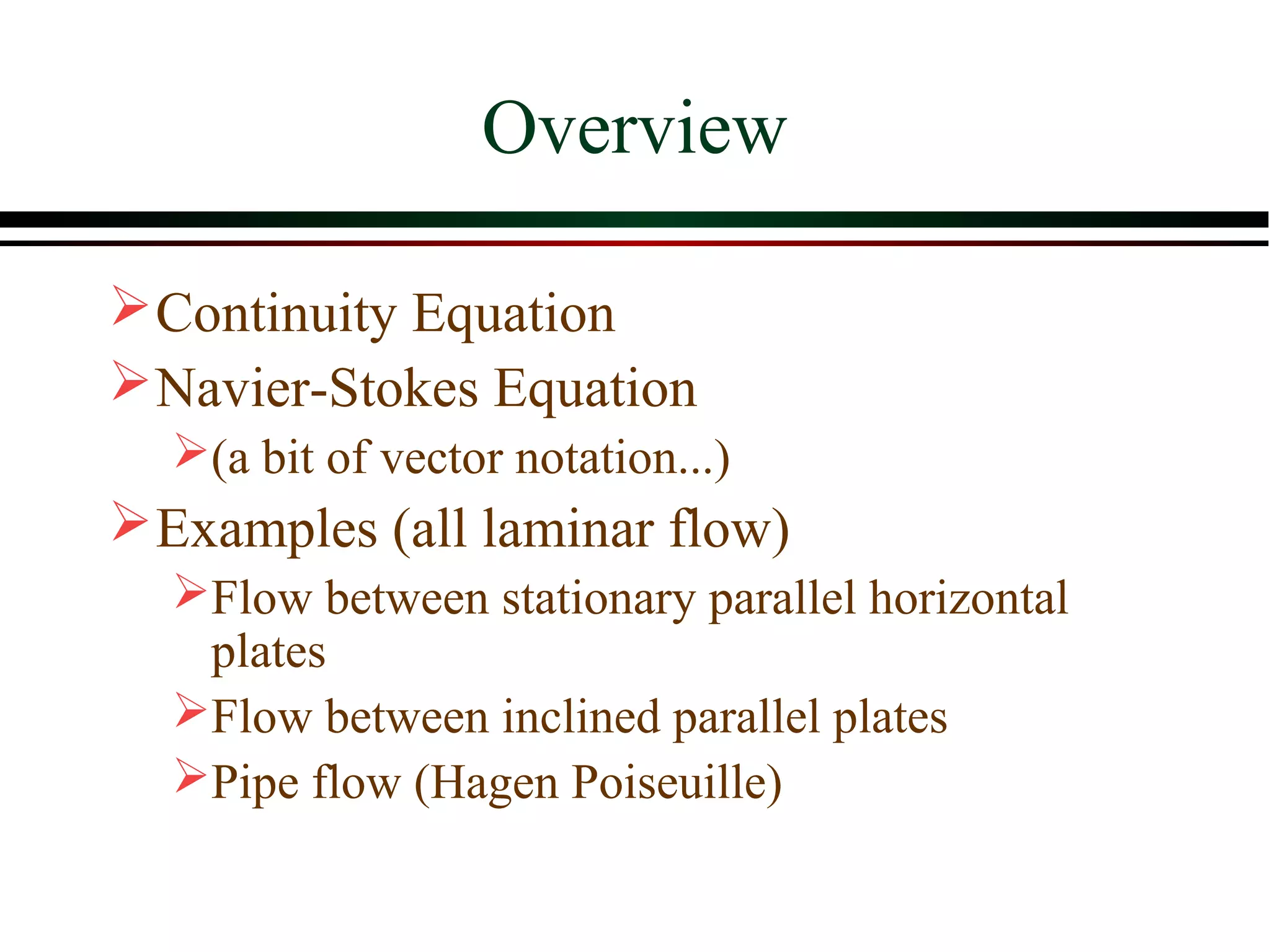
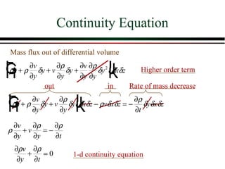
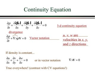
This document provides an overview of fluid dynamics concepts including the continuity equation, Navier-Stokes equations, and examples of their application to laminar flow situations. It derives the 1-dimensional continuity equation and uses it to describe flow between parallel plates. It then derives the equation for laminar flow velocity profile between infinite horizontal parallel plates based on the Navier-Stokes equations and applies it to calculate discharge rate. Finally, it provides an example problem calculating discharge rate and power for an oil skimming device.


