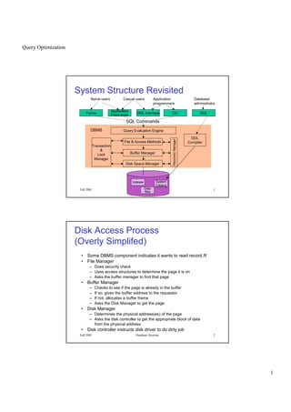
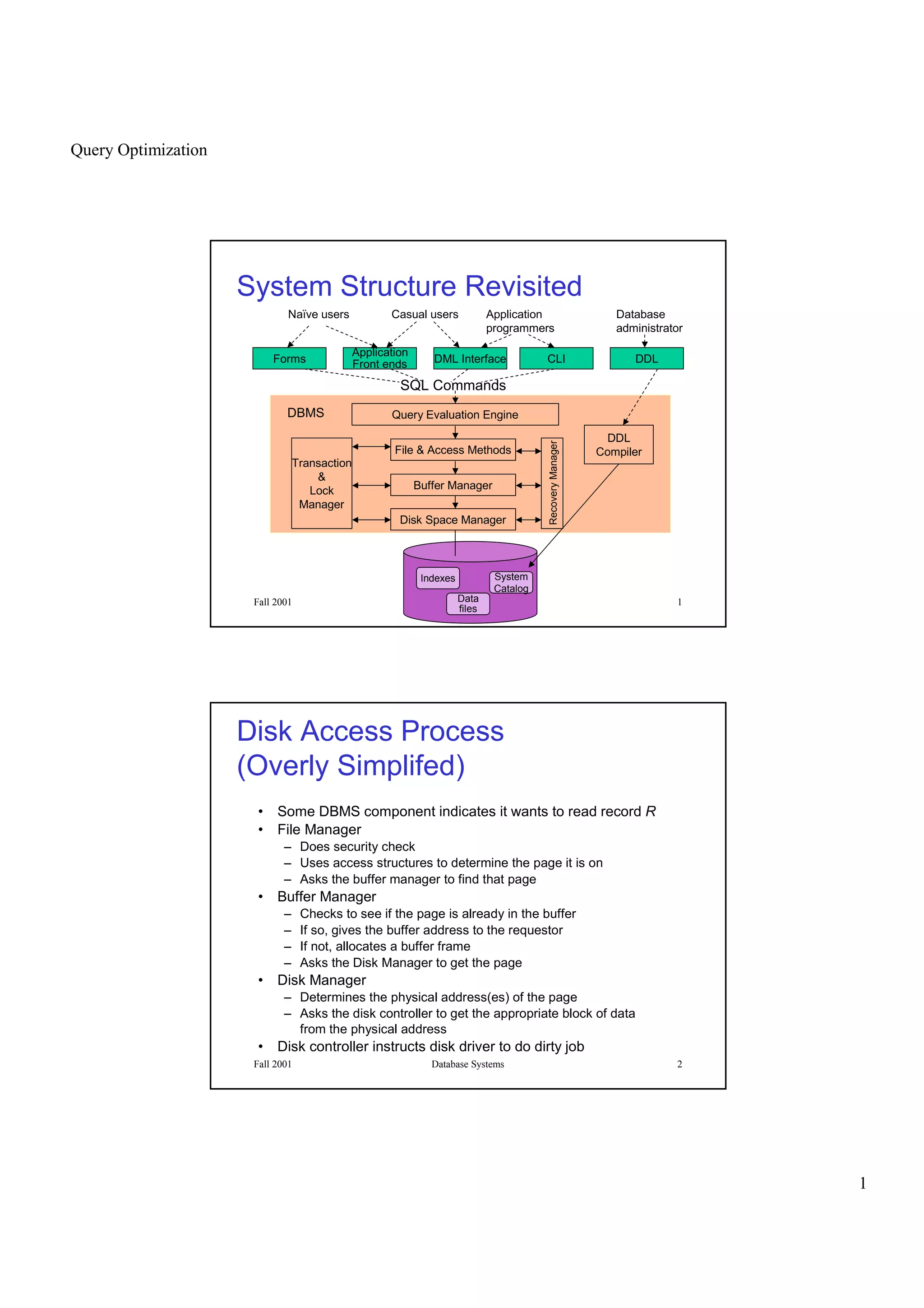
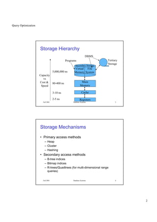
This document discusses query optimization in database systems. It begins by describing the components of a database management system and how queries are processed. It then explains that the goal of query optimization is to reduce the execution cost of a query by choosing efficient access methods and ordering operations. The document outlines different query plans involving table scans, index scans, and joins. It also introduces concepts like filter factors, statistics about tables and indexes, and how these are used to estimate the cost of alternative query execution plans.

1. Query Optimization
1
Fall 2001 Database Systems 1
System Structure Revisited
Naïve users Application
programmers
Casual users Database
administrator
Forms
Application
Front ends DML Interface CLI DDL
Indexes System
Catalog
Data
files
DDL
Compiler
Disk Space Manager
Buffer Manager
File & Access Methods
Query Evaluation Engine
SQL Commands
RecoveryManager
Transaction
&
Lock
Manager
DBMS
Fall 2001 Database Systems 2
• Some DBMS component indicates it wants to read record R
• File Manager
– Does security check
– Uses access structures to determine the page it is on
– Asks the buffer manager to find that page
• Buffer Manager
– Checks to see if the page is already in the buffer
– If so, gives the buffer address to the requestor
– If not, allocates a buffer frame
– Asks the Disk Manager to get the page
• Disk Manager
– Determines the physical address(es) of the page
– Asks the disk controller to get the appropriate block of data
from the physical address
• Disk controller instructs disk driver to do dirty job
Disk Access Process
(Overly Simplifed)

2. Query Optimization
2
Fall 2001 Database Systems 3
Storage Hierarchy
Cache
Main
Memory
Virtual
Memory
File
System
Tertiary
Storage
Programs
DBMS
Capacity
vs
Cost &
Speed
Secondary Storage
Registers2-5 ns
3-10 ns
80-400 ns
5,000,000 ns
Fall 2001 Database Systems 4
Storage Mechanisms
• Primary access methods
– Heap
– Cluster
– Hashing
• Secondary access methods
– B-tree indices
– Bitmap indices
– R-trees/Quadtrees (for multi-dimensional range
queries)

3. Query Optimization
3
Fall 2001 Database Systems 5
Query Optimization
• The goal of query optimization is to reduce the
execution cost of a query
• It involves:
– checking syntax
– simplifying the query
– execution:
• choosing a set of algorithms to execute
choosing a set of access methods for
relations
• ordering the query steps
– creating executable code to process the query
Fall 2001 Database Systems 6
Query Resource Utilization
• An optimizer must have an objective function
• Optimize the use of resources:
– CPU time
– I/O time
– number of remote calls (amount of remote data
transfer)
• Define an objective function
– c1 * costI/O(execution plan) + c2 * costCPU (execution
plan)
– many systems assume CPU costs are directly
proportional to I/O costs and optimize for costI/O only

4. Query Optimization
4
Fall 2001 Database Systems 7
Query Plan
• A query plan consists of
– methods to access relations (sequential
scan, index scan)
– methods to perform basic operations (hash
join/merge-sort join)
– ordering of these operations
– other considerations (writing temporary
results to disk, remote calls, sorting, etc.)
Fall 2001 Database Systems 8
Main query operations
• SELECT (WHERE C)
– Scan a relation and find tuples that satisfy a condition C
– Use indices to find which tuples will satisfy C
• JOIN
– Join multiple relations into a single relation
• SORT/GROUP BY/DISTINCT/UNION
– Order tuples with respect to some criteria
• Note that projection can usually be performed on the fly.

5. Query Optimization
5
Fall 2001 Database Systems 9
Table Scans
• A table scan consists of reading all the disk pages in a relation
• For example:
SELECT A.StageName FROM movies.actors A
WHERE A.age < 25
Plan: read all pages in the relation one by one
for all tuples check if A.age < 25 is true
if it is true, output the tuple to some output buffer
Assume I/O is the bottleneck
Key question is how fast can I read the whole relation?
I/O
CPU
Fall 2001 Database Systems 10
Table Scan
• A fast disk read:
– seek time 4.9 ms
– rotational latency 2.99ms
– transfer time 300 Mbits/sec
– a page of 4K is transferred in 0.1 ms
• A relation with 1 million tuples and 10 tuples per page
has:
1,000,000 / 10 = 100,000 disk pages
• A random read assumes the disk head moves to a
random location on the disk at each read:
100,000 * (4.9+2.99+0.1) = 799 sec = 13 mins

6. Query Optimization
6
Fall 2001 Database Systems 11
I/O Parallelism
• Distribute the data to multiple disks (striping)
– distribute uniformly to allow all disk heads to work equally
hard
– introduce fault tolerance
• In the best case, n disks may give a speed up factor of n
– but the total load is the same
– the cost of the system may have increased!
Page 1, 5,
9, 13, ...
Page 2, 6,
10, ...
Page 3, 7,
11, ...
Page 4, 8,
12, ...
Fall 2001 Database Systems 12
Other Scan Speed-Ups
• Read multiple pages and then perform logic filter operations
– sequential prefetch (read k consecutive pages at once)
– list prefetch (read k pages in a list at once, let the disk arm
scheduler find the optimal way of reading them)
• Example (sequential prefetch)
– read 32 pages at once and pay seek time and rotational latency
only once
4.9 + 2.99 + 0.1*32 = 11.09 ms
– to read 100,000 disk pages, make 100,000 / 32 read rounds
(each takes 11.09 ms = 11.09/1000 sec)
– total read time is then 11.09/1000 * 100,000/32 = 34.6 sec

7. Query Optimization
7
Fall 2001 Database Systems 13
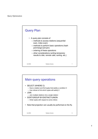
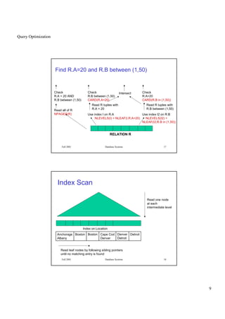
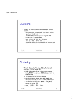
SELECT * FROM T WHERE P
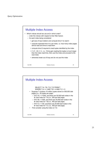
• Table scan methods
– read the entire table and select tuples that satisfy
the predicate P [sequential scan]
– prefetching is used to reduce the read time (read
blocks of N pages at once from the same track)
[sequential scan with prefetch]
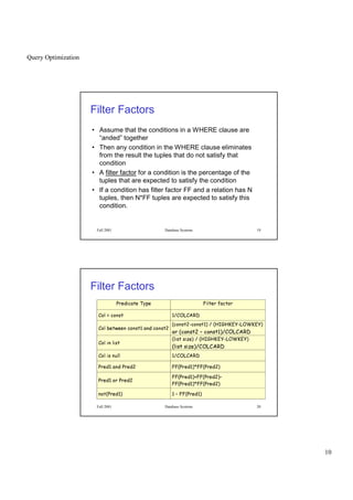
• Index scan methods
– use indices to find tuples that satisfy all of P and
then read the tuples from disk [index scan]
– use indices to find tuples that satisfy part of P and
then read the tuples from disk and check the rest
of P [index scan+select]
Fall 2001 Database Systems 14
SELECT * FROM T WHERE P
• Index scan methods (continued)
– use indices to find tuples that satisfy all of P and output the
indexed attributes [index-only scan]
– use indices to find tuples that satisfy part of P and then find the
intersection of different sets of tuples [multi-index scan]

8. Query Optimization
8
Fall 2001 Database Systems 15
Statistics in Oracle
ANALYZE TABLE employee
COMPUTE STATISTICS FOR COLUMNS dept, name
• For each relation:
– CARD: total number of tuples in the relation (cardinality)
– NPAGES: total number of disk pages for the relation
• For each column:
– COLCARD: number of distinct values for that column
– HIGHKEY, LOWKEY: the highest and the lowest stored
value for that column
In addition we will use: CARD(R WHERE C) to denote the
number of tuples in R that satisfy the condition C
Fall 2001 Database Systems 16
Statistics in Oracle
ANALYZE TABLE employee
COMPUTE STATISTICS FOR COLUMNS dept,
name
• For each index:
– NLEVELS: number of levels of the B+-tree
– NLEAF: total number of leaf pages
– FULLKEYCARD: total number of distinct values for
the index column
– CLUSTER-RATIO: percentage of rows in the table
clustered with respect to the index column

9. Query Optimization
9
Fall 2001 Database Systems 17
Find R.A=20 and R.B between (1,50)
RELATION R
Read all of R
NPAGES(R)
Check
R.A = 20 AND
R.B between (1,50)
Use index I on R.A
NLEVELS(I) + NLEAF(I,R.A=20)
Read R tuples with
R.A = 20
Check
R.B between (1,50)
CARD(R.A=20)
Use index I2 on R.B
NLEVELS(I2) +
NLEAF(I2,R.B in (1,50))
Read R tuples with
R.B between (1,50)
Check
R.A=20
CARD(R.B in (1,50))
Intersect
Fall 2001 Database Systems 18
Index Scan
Read one node
at each
intermediate level
Read leaf nodes by following sibling pointers
until no matching entry is found
Index on Location
Boston Boston Cape Cod
Denver
Anchorage
Albany
Denver
Detroit
Detroit

10. Query Optimization
10
Fall 2001 Database Systems 19
Filter Factors
• Assume that the conditions in a WHERE clause are
“anded” together
• Then any condition in the WHERE clause eliminates
from the result the tuples that do not satisfy that
condition
• A filter factor for a condition is the percentage of the
tuples that are expected to satisfy the condition
• If a condition has filter factor FF and a relation has N
tuples, then N*FF tuples are expected to satisfy this
condition.
Fall 2001 Database Systems 20
Filter Factors
¢¡¤£¦¥¨§ ©¢£¨¦£ § £¡!#©$%¦¡
%¨$'(©)%0)1$ 243 ¨576#¨8@9BA
%¨¢C¢£¦)DE£#£0F©)%¦01$$2G¦0¥©)%¦01IH P
©%¦01$$HQ4©)%0)1I24RE3
PTS@U#VWSYX`ba
Q 6¦5Yc
X`ba
R
d¨egfih#dp#q#r¦sutvh#dp#q#rwyx€¦‚„ƒ†…‚„‡(ˆ‰
%¨¢§ 0g § 1$ P
§ 1‘1¢§ ’$£bRG3
PTS@U#VWSYX`ba
Q 6b5Yc
X¦`ba
R
f“ ” q#rgq¨” •b–¨x4€b‚Wƒv…‚W‡Fˆ@‰
%¨¢§ 1(0$—¦ 243 ¨576#¨8@9BA
#¡¤£¦¥¨2„b0$¥† ¢¡¤£¦¥¨H ˜
P
¢¡£¦¥¨2iR ™˜˜
P
¢¡¤£¦¥dHbR
#¡¤£¦¥¨2„%b¡‘ ¢¡¤£¦¥dH
˜
P
¢¡£¦¥¨2iRfe¢˜
P
¢¡¤£¦¥dHbRfg
˜
P
¢¡£¦¥¨2iR ™˜˜
P
¢¡¤£¦¥dHbR
0)%#
P
¢¡¤£¦¥d24R 2GgF˜
P
¢¡¤£¦¥d24R

11. Query Optimization
11
Fall 2001 Database Systems 21
Filter factors
• Filter factors assume uniform distribution of values and no
correlation between attributes
• Suppose that we are storing the transactions of customers
at different Hollywood Video stores.
• Attributes: store_zipcode, movieid, customer_name,
customer_zipcode, date_rented
– 40,000 store_zipcodes between 10,000 and 50,000
– 10,000 movies ids between 1 and 10,000
– 100,000 customer_names between 1 and 100,000
– 40,000 customer_zipcodes between 10,000 and 50,000
– 364 dates (between 1 and 364)
– Total cardinality: 300 billion tuples
Fall 2001 Database Systems 22
Filter Factors
• What are the filter factors of the following conditions?
– All tuples for the customers named “John Smith”
– All tuples for the customers living in 12180
– All tuples for the stores located in 12180
– All tuples for the rentals on day 200
1/COLCARD = 1/100,000 = 0.00001
1/COLCARD = 1/40,000 = 0.000025
1/COLCARD = 1/40,000 = 0.000025
1/COLCARD = 1/364 = 0.0027

12. Query Optimization
12
Fall 2001 Database Systems 23
Filter Factors
– All tuples for the rentals on days (200,210,220) AND
by customer named “John Smith”
– All tuples for the rentals on day 200 AND in a store
with zipcode between 12000 and 14000
– All tuples for the rentals on day 200 OR by a
customer living in zipcode 12180
– All tuples for a customer NOT living 12180
3/363 * 1/100,000 = .0083 * .00001 = .000000083
.0027 * 2000/40,000 = .0027 * .05 = .000135
.0027 + .000025 – (.0027)(.000025) = .002724933
1 – FF(customer in 12180) = 1 - .000025 = .999975
Fall 2001 Database Systems 24
Matching Index Scan
SELECT I.name FROM items I WHERE I.location = ‘Boston’
• Assume B+-tree index ILoc on items.location
• Algorithm:
scan index for leftmost leaf where location = ‘Boston’
for all rowids R found in the leaf
retrieve tuple from items using R
find next leaf node with location = ‘Boston’ and repeat
• Cost: reading from B+-tree + reading the tuples from items
NLEVELS(Iloc) + NLEAF(Iloc, I.location=‘Boston’) + CARD(I.location=‘Boston’)
• Assume non-leaf nodes of B+-tree are already in memory and leaf
nodes store at most 400 rowids
• To retrieve n tuples, we need n / 400 + n disk accesses in the average
case

13. Query Optimization
13
Fall 2001 Database Systems 25
Partial-Matching Index Scan
SELECT I.name FROM items I
WHERE I.location = ‘Boston’ AND I.name like ‘Antique%’
• Assume B+-tree index on items.location
• Algorithm:
scan index for leftmost leaf where location = ‘Boston’
for all rowids R found in the leaf
retrieve the tuple from items using R
check if the name is like ‘Antique%’
find next leaf node with location = ‘Boston’ and repeat
• Except for some additional CPU cost, the cost of this scan is
identical to the previous one
Fall 2001 Database Systems 26
Matching Index Scan
SELECT I.name FROM items I
WHERE I.location = ‘Boston’ AND I.name like ‘Antique%’
• Assume B+-tree index IL on items.location, index IN on items.name, and
index ILN on items.location+items.name
• Options:
PLAN1: Use index IL, read the items tuples and filter on items.name
(previous slide)
PLAN2: Use index IN, read the items tuples and filter on items.location
PLAN3: Use index IL to find tuple ids SL, use index IN to find tuple ids
SN, compute intersection of SL and SN, and read the items tuples
from disk that are in this intersection
PLAN4: Use index ILN to find tuples with values Boston+Antique%.
Return the name value of all tuples from ILN that match the criteria
(Index only scan)

14. Query Optimization
14
Fall 2001 Database Systems 27
Comparing Costs (1)
• Assume items contains 1 million tuples, 50 different
cities and 100,000 different names for items
• Assume B+-trees can store at most 400 duplicate
values per node at the leaf level
• The items table can store about 20 tuples in a single
disk page
• If we assume uniform distribution, there are
– 1M / 50 = 20,000 items in Boston
– 1M / 100,000 = 10 items of each different name
– assume 100 names start with Antique so that 1000
items have a name like ‘Antique%’
Fall 2001 Database Systems 28
Comparing Costs (2)
• B+-tree indices
– Index IL: items from Boston are stored in 20,000 / 400
= 50 disk pages
– Index IN: items with names that start with Antiques are
stored in 1000/400 = 3 disk pages
• Assume that only leaf nodes of a B+-Tree index are read
from disk during query execution
• PLAN 1: To read all tuples for ‘Boston’ requires 50 index
pages + 20,000 pages from items = 20,050 disk reads

15. Query Optimization
15
Fall 2001 Database Systems 29
Comparing Costs (3)
• PLAN 2: To read all tuples with name like ‘Antique%’
requires 3 index pages + 1000 pages from items = 1003
disk reads
• PLAN 4: How big is the B+-tree for ILN? Assume 150
rowids at most fit in a leaf of ILN
– Assume 1 tuple for each city and name combination
– the 100 item names of the form ‘Antique%’ are stored
consecutively for a given location and fit in a single
page
– cost: read 1 B+-tree page with Boston+Antique% and
find all 100 names, so 1 disk read
Fall 2001 Database Systems 30
Indices Not Always Best
• Assume seek time 4.9 ms, latency 3.0 ms, transfer 0.1
ms/page
• Suppose we want to find all items in ‘Boston’
• Use IL index on items.location:
– 20,000 items per city, 50 index pages per city
– total cost is 20,050 disk page reads (assuming no
clustering on location)
– 20,050 * 8 = 160 sec = 2.7 min
• Sequential scan with prefetch = 32
– 1M tuples, 1M / 20 = 50,000 disk pages
– 50,000 / 32 = 1563 rounds
– 1563 * (4.9+3+3.2) = 17.35 sec

16. Query Optimization
16
Fall 2001 Database Systems 31
Clustering
• Remember, clustering means that the tuples of a relation are stored in
groups with respect to a set of attributes
• Assume BIDS(bidid,itemid,buyid,date,amount) is clustered on itemid,
buyid
– all bids for the same item are on consecutive disk pages
– all bids for the same item by the same buyer are on the same disk
page
• It is very fast to find
– all bids on a specific item
– all bids on a specific item by a specific buyer
• It is not very fast to find
– all bids by a specific buyer
– all bids of some amount
Fall 2001 Database Systems 32
Clustering
• Assume that there are 20 bids per item in general,
20 million tuples in the bids relation, and a total of
10,000 buyers
– Suppose 40 bids tuples fit on a single page
– B+-tree index IIB on itemid, buyid stores 200
rowids per page
– B+-tree index IB on buyid stores 400 rowids per
page

17. Query Optimization
17
Fall 2001 Database Systems 33
Clustering
• What is the cost of finding all bids for items I1 through
I1000?
– How many bids do we expect? 1000 items * 20 bids
per item = 20,000 bids
– 20,000 / 200 =100 index pages using index IIB
– 20,000 / 40 = 500 bids pages
– with prefetch=32, 500 / 32 = 16 rounds
– 16*(4.9+3+3.2) + 100*8 = 0.97 sec
– We might be able to use prefetch for the index as well
Fall 2001 Database Systems 34
Clustering
• What is the cost of finding all bids for items I1
through I1000 by buyer B5?
– how many bids do we expect? 20 bids per
item, 10,000 buyers, so .002 bids per item by a
given buyer
– 1000 items, so 20,000 bids total
– each bid for the same item and buyer are
stored consecutively in index IIB and on disk
– 1000 index accesses + (1000 * .002) bids
pages for buyer B5
– cost = 1000*8 + 2*8 = 8 sec

18. Query Optimization
18
Fall 2001 Database Systems 35
Clustering
• What is the cost of finding all bids by buyer B5?
– 20 bids per item / 10,000 buyers = .002 bids per
buyer on each item
– .002 bids per buyer per item * 1M items = 2000 bids
per buyer
– bids by the same buyer for different items are stored
on different pages
• if we use index IB, we need to access 2000
pages and 2000/400 = 5 index pages
• cost = 2000*8 + 5*8 = 16.04 sec
– sequential scan: 20M / 40 = 500,000 disk pages
• Use prefetch = 32, 500,000 / 32 = 15625 rounds
• 15625 * (4.9+3+3.2) = 2.9 minutes
Fall 2001 Database Systems 36
Design Process - Physical Design
Conceptual
Design
Conceptual Schema
(ER Model)
Logical
Design
Logical Schema
(Relational Model)
Physical
Design
Physical Schema

19. Query Optimization
19
Fall 2001 Database Systems 37
Physical Design
• Choice of indexes
• Clustering of data
• May have to revisit and refine the conceptual
and external schemas to meet performance
goals.
• Most important is to understand the workload
– The most important queries and their frequency.
– The most important updates and their frequency.
– The desired performance for these queries and
updates.
Fall 2001 Database Systems 38
Workload Modeling
• For each query in the workload:
– Which relations does it access?
– Which attributes are retrieved?
– Which attributes are involved in selection/join
conditions? How selective are these conditions
likely to be?
• For each update in the workload:
– Which attributes are involved in selection/join
conditions? How selective are these conditions
likely to be?
– The type of update (INSERT/DELETE/UPDATE),
and the attributes that are affected.

20. Query Optimization
20
Fall 2001 Database Systems 39
Physical Design Decisions
• What indexes should be created?
– Relations to index
– Field(s) to be used as the search key
– Perhaps multiple indexes?
– For each index, what kind of an index should it be?
• Clustered? Hash/tree? Dynamic/static? Dense/sparse?
• Should changes be made to the conceptual schema?
– Alternative normalized schemas
– Denormalization
– Partitioning (vertical horizontal)
– New view definitions
• Should the frequently executed queries be rewritten
to run faster?
Fall 2001 Database Systems 40
Choice of Indexes
• Consider the most important queries one-by-one
– Consider the best plan using the current indexes
– See if a better plan is possible with an additional
index
– If so, create it.
• Consider the impact on updates in the workload
– Indexes can make queries go faster,
– Updates are slower
– Indexes require disk space, too.

21. Query Optimization
21
Fall 2001 Database Systems 41
Index Selection Guidelines
• Don’t index unless it contributes to performance.
• Attributes mentioned in a WHERE clause are candidates
for index search keys.
– Exact match condition suggests hash index.
– Range query suggests tree index.
• Clustering is especially useful for range queries, although it can help
on equality queries as well in the presence of duplicates.
• Multi-attribute search keys should be considered when a
WHERE clause contains several conditions.
– If range selections are involved, order of attributes should be
carefully chosen to match the range ordering.
– Such indexes can sometimes enable index-only strategies for
important queries.
• For index-only strategies, clustering is not important!
Fall 2001 Database Systems 42
Index Selection Guidelines (cont’d.)
• Try to choose indexes that benefit as many
queries as possible. Since only one index can
be clustered per relation, choose it based on
important queries that would benefit the most
from clustering.

22. Query Optimization
22
Fall 2001 Database Systems 43
Matching composite index scans
An extent - normally read
with a sequential prefetch
Relation R
B+-tree for Relation R on
columns C1, C2, C3, C4
• Entries for the same C1, C2, C3 values (but different C4
values) are located in consecutive leaf pages
• Same for C1,C2 entries but with different C3 or C4 entries
• Matching index scan is a search for consecutively stored
leaf pages
Fall 2001 Database Systems 44
Matching composite index scans
• Hollywood Video relation: (store_zipcode, movieid,
customer_name, customer_zipcode, date_rented)
• Suppose we have a B+-tree index on store_zipcode,
customer_zipcode, movieid, date_rented, in which each
leaf node stores 200 rowids
SELECT S.customer_name
FROM Store S
WHERE S.store_zipcode = 12180 AND
S.customer_zipcode = 12180 AND
S.movie_id between 1000 and 2000
– find the leftmost leaf node with 12180, 12180, and
movie-id = 1000
– read all leaf nodes from left to right until a movie with
id2000 is found.

23. Query Optimization
23
Fall 2001 Database Systems 45
Matching composite index scans
• How many tuples do we expect in the result?
• Expected number of tuples:
FF: 1/40,000 * 1/40,000 * 1000/10,000 = 6.25 x 10-11
N = 300 billion * FF = 3 x 1011 * 6.25 x 10-11 = 19
• How many disk pages do we read?
N / 200 B+-tree nodes + N pages of the relation = 20
assumes no clustering on the STORE relation for the
store_zipcode, customer_zipcode, movie_id attributes
Fall 2001 Database Systems 46
Matching composite index scans
• Hollywood Video relation: (store_zipcode, movieid,
customer_name, customer_zipcode, date_rented)
• Suppose we have a B+-tree index on store_zipcode,
customer_zipcode, movieid, date_rented, in which each
leaf node stores 200 tuples
SELECT S.customer_name
FROM Store S
WHERE S.store_zipcode between 12180 and 42180 AND
S.customer_zipcode = 12180 AND
S.movie_id = 20
• Not a matching scan, B+-tree nodes with different
store_zipcode values for customer_zipcode 12180 are not
in consecutive leaf-nodes

24. Query Optimization
24
Fall 2001 Database Systems 47
Matching composite index scans
• How many disk pages do we expect to read if we scanned for
S.customer_zipcode = 12180 AND S.movie_id = 20 ?
– Note that these tuples are not consecutive on disk, we cannot perform
a matching index scan
• We can read the B+-tree index at the leaf level for
S.store_zipcode between 12180 and 42180 reading ¾ of the
tuples.
– Use sequential prefetch = 32:
300 billion / 200 = 1.5 billion nodes total in the B+ tree
1.5 *3/4 = 1.125 billion nodes read for the range search
1.125 billion / 32 = 35 million rounds
35 million * 11.1ms = 388.5 seconds
Fall 2001 Database Systems 48
Multiple Index Access
SELECT T.A, T.B, T.D, T.E FROM T
WHERE (T.A = 4 AND (T.B 4 OR T.C 5)) OR T.E = 10
• Assume indices on columns A, B, C, E, individually.
• Plan:
– Find the set SA of all rowids with T.A = 4
– Find the set SB of all rowids with T.B 4
– Find the set SC of all rowids with T.C 5
– Find the set SE of all rowids with T.E = 10
– Compute: (SA ∩ ( SB ∪ SC)) ∪SE
– Sort the rowids in result into lists and prefetch these lists
to read the tuples of T from disk

25. Query Optimization
25
Fall 2001 Database Systems 49
Multiple Index Access
• Which indices should we use and in which order?
– order the indices with respect to their filter factors
– for each index being considered
• get size of input relation and compute time t1 to read it
• compute expected time ti to use index, i.e. how many index pages
will be read and time to read them
• compute time t2 required to read tuples identified by the index
• if (t1 - t2) ti , i.e. if time gain reading the tuples is much larger
than the index read time, then use this index and proceed to the
next index
• otherwise break out of loop and do not use this index
Fall 2001 Database Systems 50
Multiple Index Access
SELECT T.A, T.B, T.D, T.E FROM T
WHERE T.A = 4 AND T.B 4 AND T.C 5
• Suppose T contains 10 million tuples stored on 500,000 disk
pages (i.e., 20 tuples per page)
– FF(T.A) = 1/1000, and there are 50,000 leaf nodes in the
B+-tree index for T.A (i.e., 200 per leaf page)
– FF(T.B) = 1/200, and there are 25,000 leaf nodes in the
B+-tree index for T.B (i.e., 400 per leaf page)
– FF(T.C) = 1/20, and there are 25,000 leaf nodes in the
B+-tree index for T.C (i.e., 400 per leaf page)
• First consider using the index on T.A

26. Query Optimization
26
Fall 2001 Database Systems 51
Do We Use T.A Index?
• Without using index on T.A, we have to read 500,000 pages
– with a sequential prefetch of 0.01 sec per 32 pages, it will
take about 156 secs
• If index is used to find tuples with T.A = 4, we need to retrieve
50,000/1000 = 50 pages
– with a sequential prefetch of 0.01 sec per 32 pages, it will
take = 0.02 secs to read the index
– the result will have an estimated 10 million/1000 = 10,000
tuples in 10,000 different pages in the worst case
– with random I/O of 0.008 sec/page, it will take 80 secs to
read the tuples
• We gain 76 seconds by using the index
Fall 2001 Database Systems 52
Do We Use Index on T.B?
• Without using index on T.B, we have to read 10,000 pages
– with random I/O of 0.008 sec/page, it will take 80 secs
• If index is used to find tuples with T.B 4, we need to retrieve 3 *
(25,000 / 200) = 375 pages
– with a sequential prefetch of 0.01 sec per 32 pages, it will
take 0.12 secs
• The result will have an estimated 3*(10,000/200) = 150 tuples
which are on 150 different pages in the worst case
– with random I/O of 0.008 sec/page, it will take 1.2 secs to
read them
• We gain 78.7 seconds using the index for T.B

27. Query Optimization
27
Fall 2001 Database Systems 53
Do We Use Index for T.C?
• Without using index on T.C, we have to read 150 pages in
1.2 secs
• If index is used to find tuples with T.C 5, we have to read
15 * (25,000 / 20) = 18,750 pages
– with a sequential prefetch of 0.01 sec per 32 pages, it will
take = 5.86 secs
• The result will have an estimated 15 * 150 / 20 = 112.5
tuples which are on 113 different pages in the worst case
– with random I/O of 0.008 sec/page, it will take 0.904 secs
• We gain 1.2 - 0.9 = 0.3 seconds by paying 5.86 seconds to
use the index. Hence, using T.C will not pay off