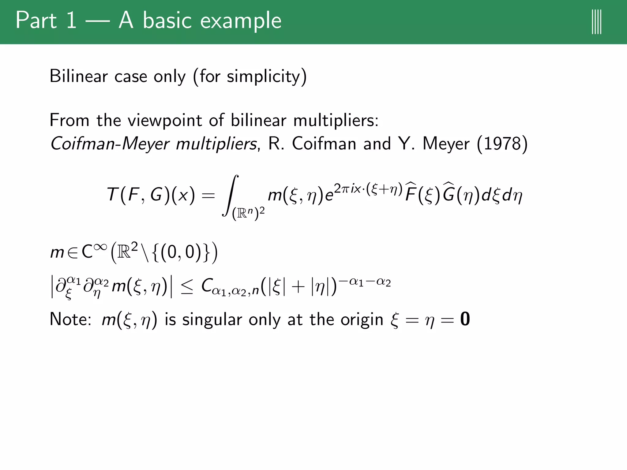
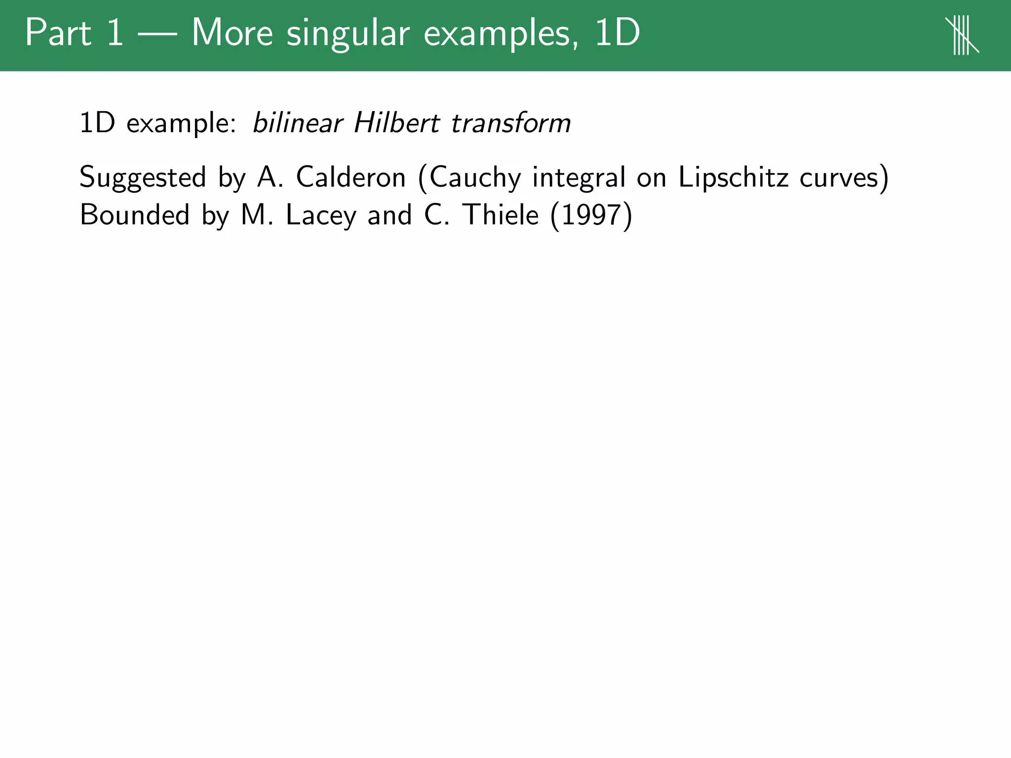
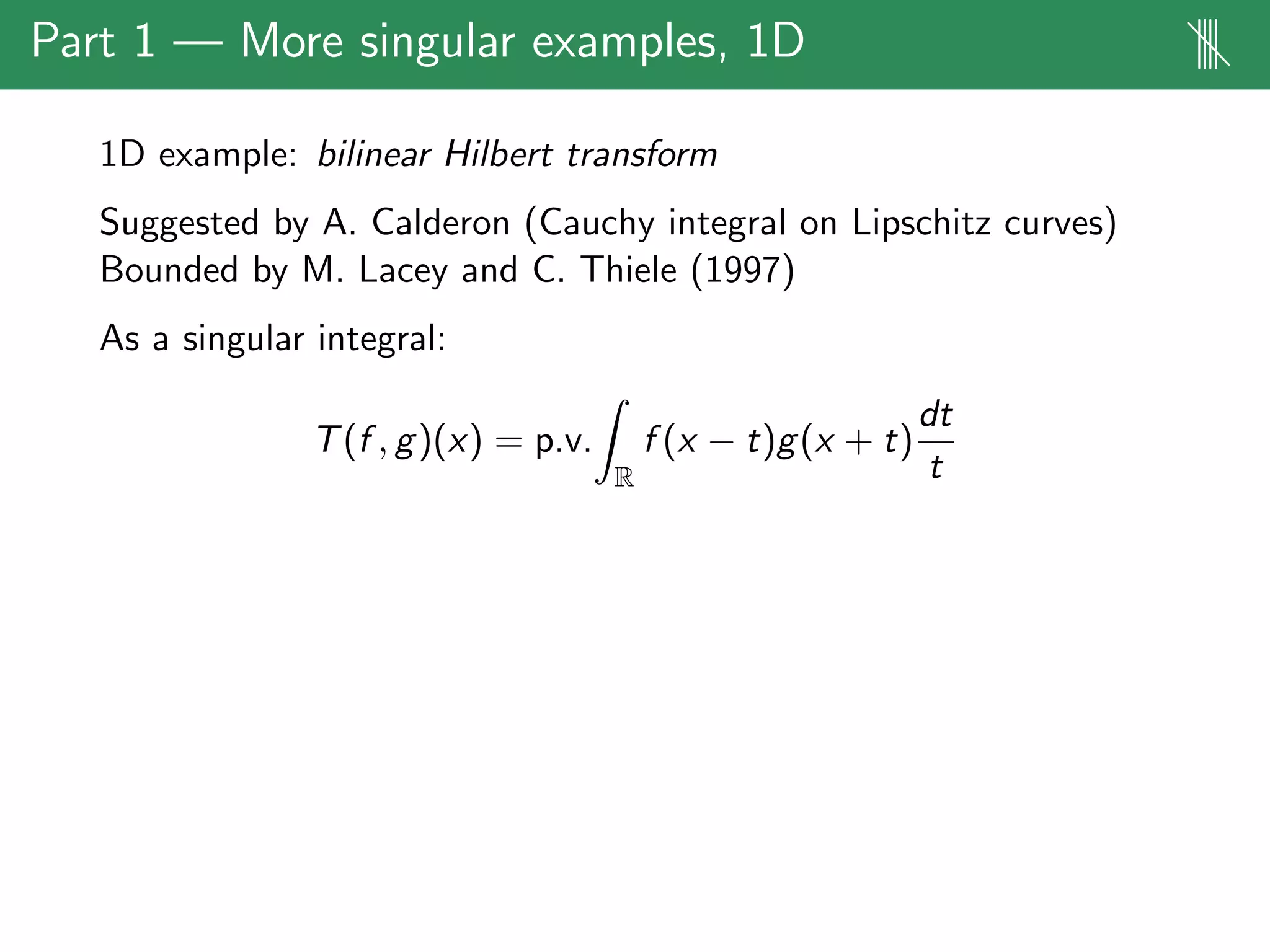
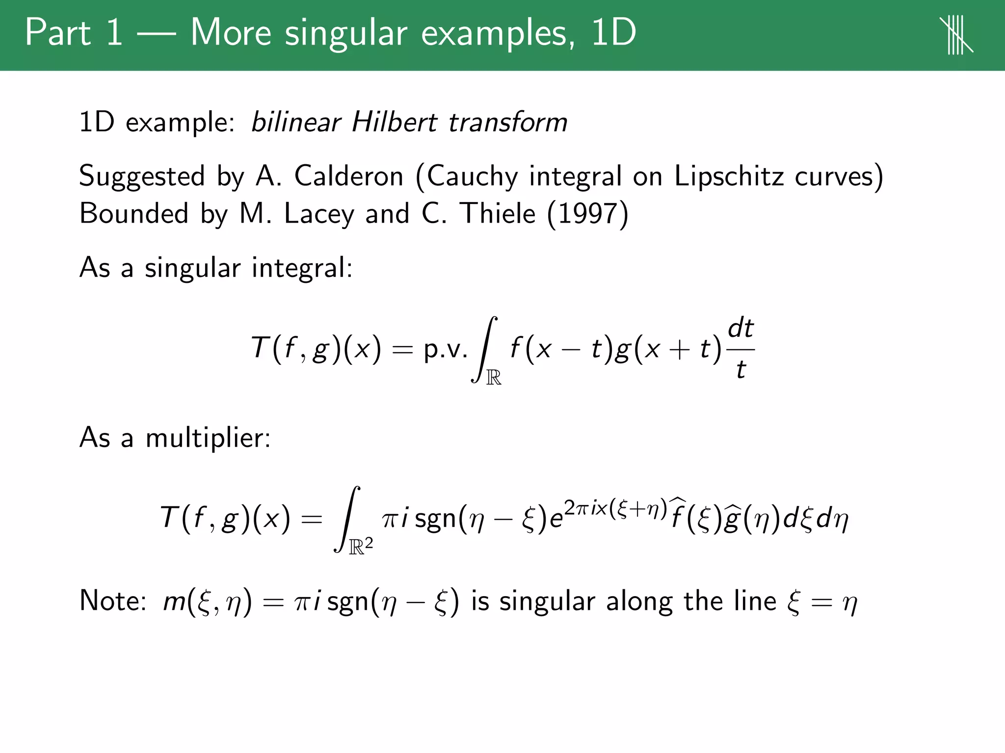
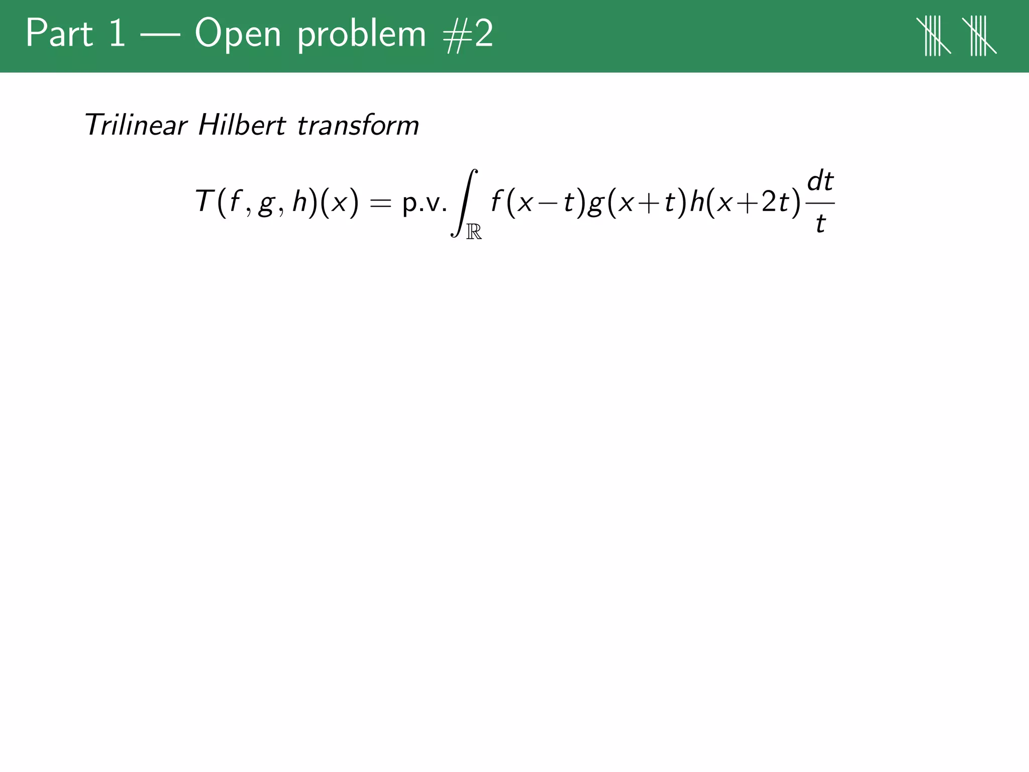
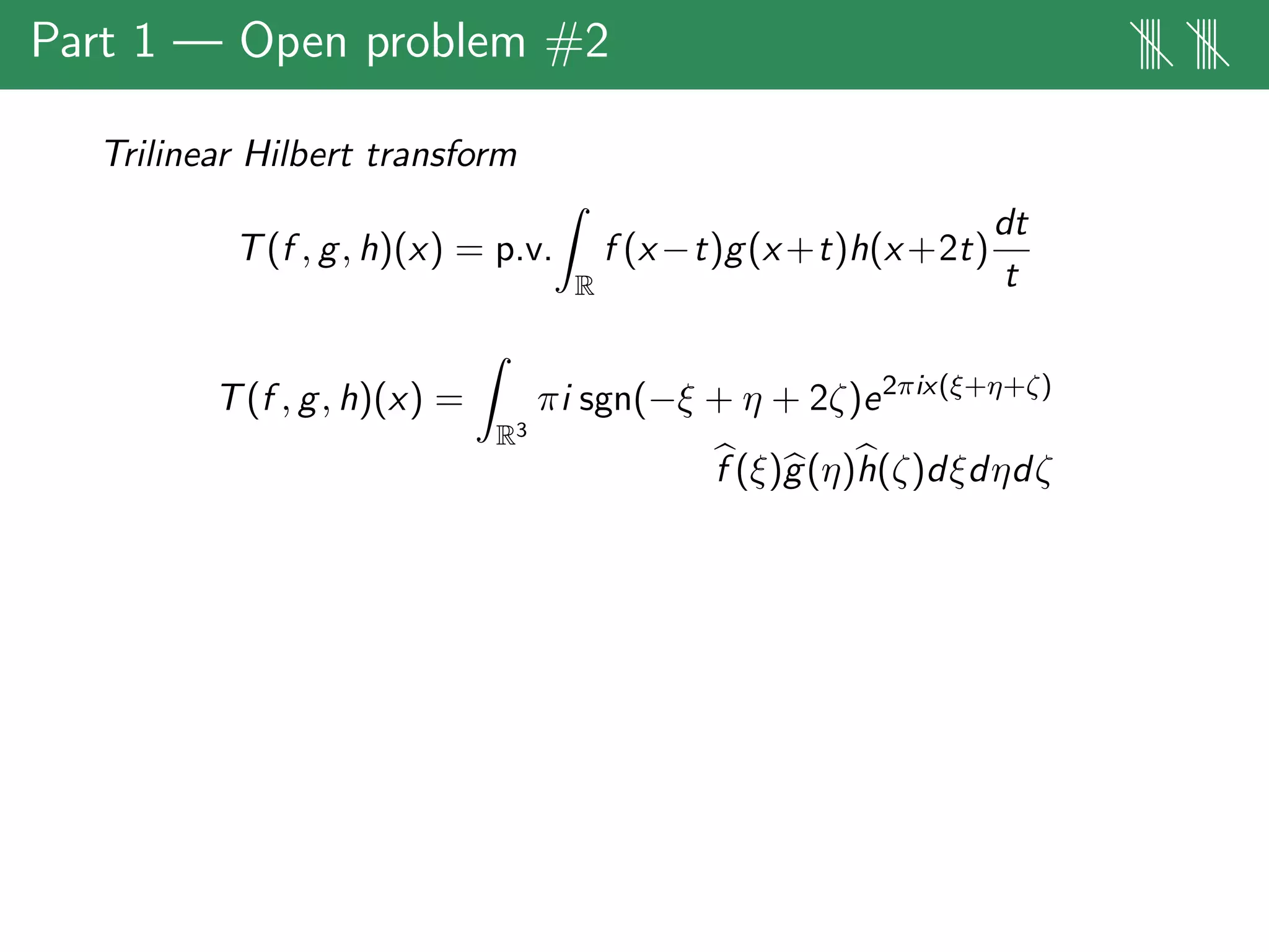
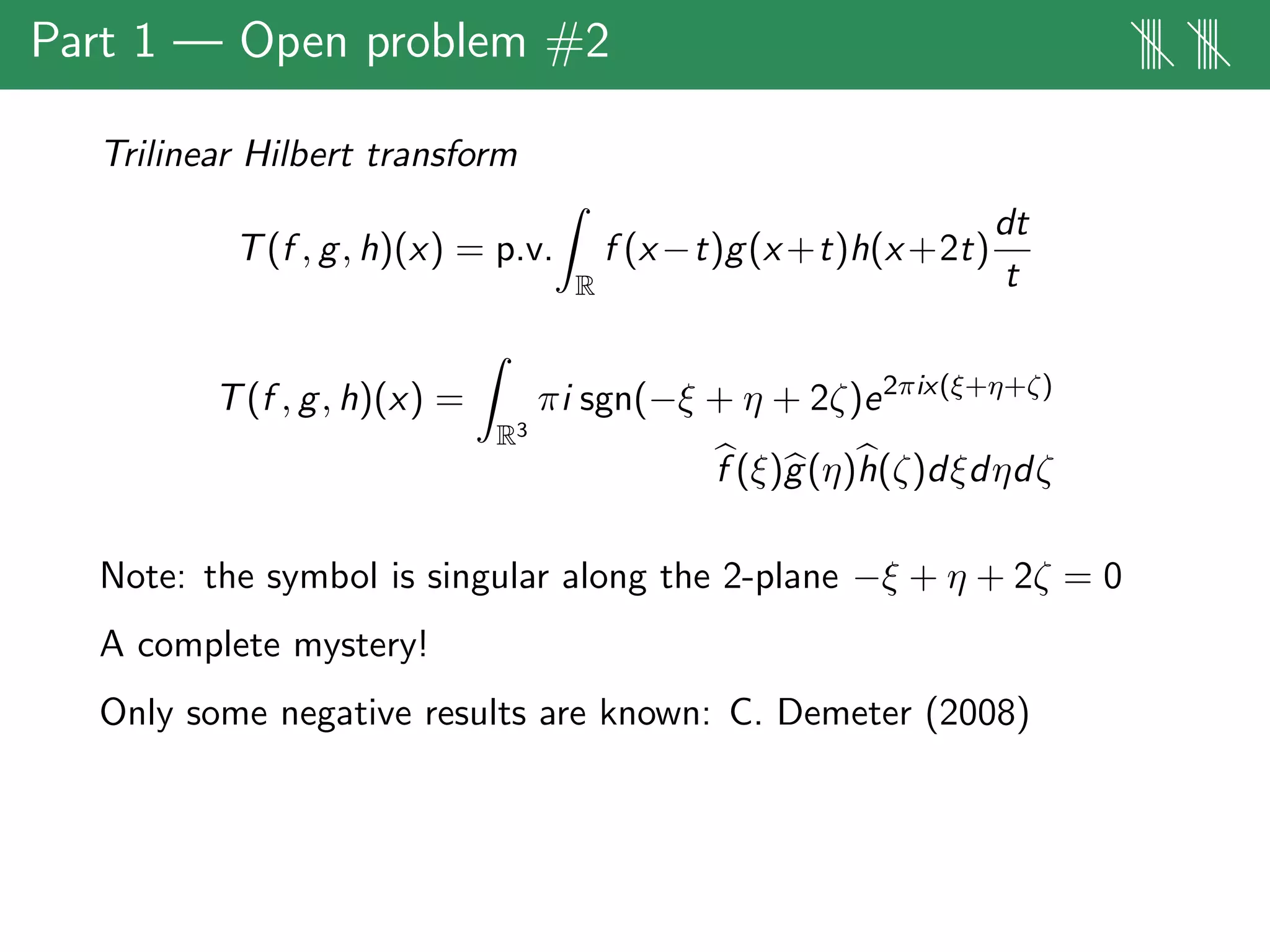
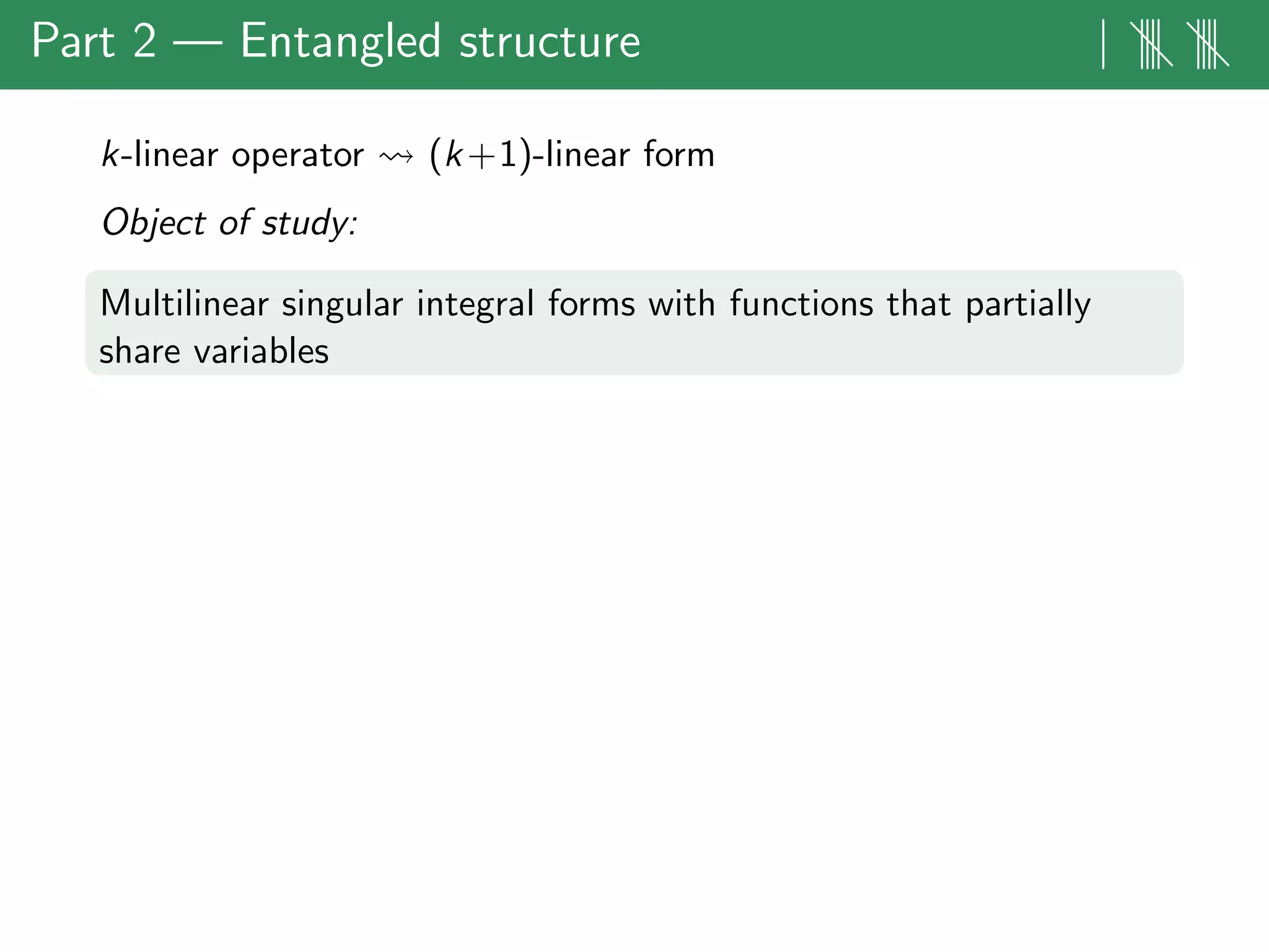
The document discusses estimates for non-standard bilinear multipliers, presenting various results and motivations for multilinear estimates and techniques. It covers the transition from dyadic model operators to continuous-type operators, as well as examples of bilinear and trilinear Hilbert transforms. The talk emphasizes open problems in the field and the complex structures involved in multilinear singular integral forms.

1. Estimates for a class of
non-standard bilinear multipliers
Vjekoslav Kovaˇc (University of Zagreb)
Joint work with Fr´ed´eric Bernicot (Universit´e de Nantes)
and Christoph Thiele (Universit¨at Bonn)
Joint CRM-ISAAC Conference on
Fourier Analysis and Approximation Theory
Bellaterra, November 6, 2013

2. Talk outline |
Part 1 — Introduction
Motivation for multilinear estimates
Concrete examples and some results

3. Talk outline |
Part 1 — Introduction
Motivation for multilinear estimates
Concrete examples and some results
Part 2 — The “entangled” structure
The scope of our techniques

4. Talk outline |
Part 1 — Introduction
Motivation for multilinear estimates
Concrete examples and some results
Part 2 — The “entangled” structure
The scope of our techniques
Part 3 — Dyadic model operators
Formulating a T(1)-type theorem
Setting up the Bellman function scheme

5. Talk outline |
Part 1 — Introduction
Motivation for multilinear estimates
Concrete examples and some results
Part 2 — The “entangled” structure
The scope of our techniques
Part 3 — Dyadic model operators
Formulating a T(1)-type theorem
Setting up the Bellman function scheme
Part 4 — Transition to continuous-type operators
Back to bilinear multipliers
“Entangled” operators with continuous kernels

6. Part 1 — Multilinear estimates ||
T = a multilinear integral operator
T is “singular” in some sense

7. Part 1 — Multilinear estimates ||
T = a multilinear integral operator
T is “singular” in some sense
We are interested in Lp
estimates:
T(F1, F2, . . . , Fk) Lp(Rn) ≤ Cp,p1,...,pk
k
j=1
Fj L
pj (R
nj )
in a subrange of 0 < p, p1, . . . , pk < ∞
Possibly also some Sobolev norm estimates, etc.

8. Part 1 — Multilinear estimates, motivation |||
Motivation for multilinear estimates:

9. Part 1 — Multilinear estimates, motivation |||
Motivation for multilinear estimates:
paraproducts
J.-M. Bony (1981) — paradifferential operators
G. David and J.-L. Journ´e (1984) — T(1) theorem

10. Part 1 — Multilinear estimates, motivation |||
Motivation for multilinear estimates:
paraproducts
J.-M. Bony (1981) — paradifferential operators
G. David and J.-L. Journ´e (1984) — T(1) theorem
multilinear expansions of nonlinear/“curved” operators
A. Calder´on (1960s) — Cauchy integral on Lipschitz curves
M. Christ and A. Kiselev (2001) — Hausdorff-Young
inequalities for the Dirac scattering transform
J. Bourgain and L. Guth (2010) — restriction estimates,
oscillatory integrals

11. Part 1 — Multilinear estimates, motivation |||
Motivation for multilinear estimates:
paraproducts
J.-M. Bony (1981) — paradifferential operators
G. David and J.-L. Journ´e (1984) — T(1) theorem
multilinear expansions of nonlinear/“curved” operators
A. Calder´on (1960s) — Cauchy integral on Lipschitz curves
M. Christ and A. Kiselev (2001) — Hausdorff-Young
inequalities for the Dirac scattering transform
J. Bourgain and L. Guth (2010) — restriction estimates,
oscillatory integrals
recurrence in ergodic theory
J. Bourgain (1988) — return times theorem
C. Demeter, M. Lacey, T. Tao, and C. Thiele (2008) —
extending the exponent range

12. Part 1 — A basic example ||||
Bilinear case only (for simplicity)

13. Part 1 — A basic example ||||
Bilinear case only (for simplicity)
From the viewpoint of bilinear singular integrals:
T(F, G)(x) = p.v.
(Rn)2
K(s, t)F(x − s)G(x − t) ds dt
K = translation-invariant Calder´on-Zygmund kernel
Generalized by L. Grafakos and R. H. Torres (2002):
multilinear C-Z operators
Take m = K

14. Part 1 — A basic example ||||
Bilinear case only (for simplicity)
From the viewpoint of bilinear multipliers:
Coifman-Meyer multipliers, R. Coifman and Y. Meyer (1978)
T(F, G)(x) =
(Rn)2
m(ξ, η)e2πix·(ξ+η)
F(ξ)G(η)dξdη
m∈C∞
R2{(0, 0)}
∂α1
ξ ∂α2
η m(ξ, η) ≤ Cα1,α2,n(|ξ| + |η|)−α1−α2
Note: m(ξ, η) is singular only at the origin ξ = η = 0

15. Part 1 — More singular examples, 1D ||||
1D example: bilinear Hilbert transform
Suggested by A. Calderon (Cauchy integral on Lipschitz curves)
Bounded by M. Lacey and C. Thiele (1997)

16. Part 1 — More singular examples, 1D ||||
1D example: bilinear Hilbert transform
Suggested by A. Calderon (Cauchy integral on Lipschitz curves)
Bounded by M. Lacey and C. Thiele (1997)
As a singular integral:
T(f , g)(x) = p.v.
R
f (x − t)g(x + t)
dt
t

17. Part 1 — More singular examples, 1D ||||
1D example: bilinear Hilbert transform
Suggested by A. Calderon (Cauchy integral on Lipschitz curves)
Bounded by M. Lacey and C. Thiele (1997)
As a singular integral:
T(f , g)(x) = p.v.
R
f (x − t)g(x + t)
dt
t
As a multiplier:
T(f , g)(x) =
R2
πi sgn(η − ξ)e2πix(ξ+η)
f (ξ)g(η)dξdη
Note: m(ξ, η) = πi sgn(η − ξ) is singular along the line ξ = η

18. Part 1 — More singular examples, 2D | ||||
2D example: a variant of the 2D bilinear Hilbert transform
Introduced by Demeter and Thiele and bounded for “most” cases
of A, B ∈ M2(R) (2008)

19. Part 1 — More singular examples, 2D | ||||
2D example: a variant of the 2D bilinear Hilbert transform
Introduced by Demeter and Thiele and bounded for “most” cases
of A, B ∈ M2(R) (2008)
As a singular integral:
T(F, G)(x, y) = p.v.
R2
K(s, t)F (x, y)−A(s, t)
G (x, y)−B(s, t) ds dt

20. Part 1 — More singular examples, 2D | ||||
2D example: a variant of the 2D bilinear Hilbert transform
Introduced by Demeter and Thiele and bounded for “most” cases
of A, B ∈ M2(R) (2008)
As a singular integral:
T(F, G)(x, y) = p.v.
R2
K(s, t)F (x, y)−A(s, t)
G (x, y)−B(s, t) ds dt
Essentially the only case that was left out:
A =
1 0
0 0
and B =
0 0
0 1

21. Part 1 — More singular examples, 2D | ||||
2D example: a variant of the 2D bilinear Hilbert transform
As a multiplier:
T(F, G)(x, y) =
R4
µ(ξ1, ξ2, η1, η2)e2πi(x(ξ1+η1)+y(ξ2+η2))
F(ξ1, ξ2)G(η1, η2) dξ1dξ2dη1dη2
µ(ξ1, ξ2, η1, η2) = m Aτ (ξ1, ξ2) + Bτ (η1, η2) , m = K
m ∈ C∞
R2{(0, 0)}
∂α1
τ1
∂α2
τ2
m(τ1, τ2) ≤ Cα1,α2 (|τ1| + |τ2|)−α1−α2
Note: µ(ξ1, ξ2, η1, η2) is singular along the 2-plane
Aτ (ξ1, ξ2) + Bτ (η1, η2) = (0, 0)

22. Part 1 — Remaining case of 2D BHT || ||||
T(F, G)(x, y) =
R4
m(ξ1, η2)e2πi(x(ξ1+η1)+y(ξ2+η2))
F(ξ1, ξ2)G(η1, η2)dξ1dξ2dη1dη2

23. Part 1 — Remaining case of 2D BHT || ||||
T(F, G)(x, y) =
R4
m(ξ1, η2)e2πi(x(ξ1+η1)+y(ξ2+η2))
F(ξ1, ξ2)G(η1, η2)dξ1dξ2dη1dη2
Theorem. Lp
estimate — F. Bernicot (2010), V. K. (2010)
T(F, G) Lr ≤ Cp,q,r F Lp G Lq
for 1 < p, q < ∞, 0 < r < 2, 1
p + 1
q = 1
r .

24. Part 1 — Remaining case of 2D BHT || ||||
T(F, G)(x, y) =
R4
m(ξ1, η2)e2πi(x(ξ1+η1)+y(ξ2+η2))
F(ξ1, ξ2)G(η1, η2)dξ1dξ2dη1dη2
Theorem. Lp
estimate — F. Bernicot (2010), V. K. (2010)
T(F, G) Lr ≤ Cp,q,r F Lp G Lq
for 1 < p, q < ∞, 0 < r < 2, 1
p + 1
q = 1
r .
Theorem. Sobolev estimate — F. Bernicot and V. K. (2013)
If supp m ⊆ (ξ1, η2) : |ξ1| ≤ c |η2| , then
T(F, G) Lr
y (Ws,r
x ) ≤ Cp,q,r,s F Lp G Ws,q
for s ≥ 0, 1 < p, q < ∞, 1 < r < 2, 1
p + 1
q = 1
r .

25. Part 1 — A warning example ||| ||||
Bi-parameter bilinear Hilbert transform

26. Part 1 — A warning example ||| ||||
Bi-parameter bilinear Hilbert transform
T(F, G)(x, y) = p.v.
R2
F(x − s, y − t) G(x + s, y + t)
ds
s
dt
t

27. Part 1 — A warning example ||| ||||
Bi-parameter bilinear Hilbert transform
T(F, G)(x, y) = p.v.
R2
F(x − s, y − t) G(x + s, y + t)
ds
s
dt
t
T(F, G)(x, y) =
R4
π2
sgn(ξ1 + ξ2)sgn(η1 + η2)
e2πi(x(ξ1+η1)+y(ξ2+η2))
F(ξ1, ξ2)G(η1, η2) dξ1dξ2dη1dη2

28. Part 1 — A warning example ||| ||||
Bi-parameter bilinear Hilbert transform
T(F, G)(x, y) = p.v.
R2
F(x − s, y − t) G(x + s, y + t)
ds
s
dt
t
T(F, G)(x, y) =
R4
π2
sgn(ξ1 + ξ2)sgn(η1 + η2)
e2πi(x(ξ1+η1)+y(ξ2+η2))
F(ξ1, ξ2)G(η1, η2) dξ1dξ2dη1dη2
Satisfies no Lp
estimates!
C. Muscalu, J. Pipher, T. Tao, and C. Thiele (2004)
Note: the symbol is singular along the union of two 3-planes,
ξ1 + ξ2 = 0 and η1 + η2 = 0

29. Part 1 — Open problem #1 |||| ||||
Triangular Hilbert transform

30. Part 1 — Open problem #1 |||| ||||
Triangular Hilbert transform
T(F, G)(x, y) = p.v.
R
F(x−t, y)G(x, y −t)
dt
t

31. Part 1 — Open problem #1 |||| ||||
Triangular Hilbert transform
T(F, G)(x, y) = p.v.
R
F(x−t, y)G(x, y −t)
dt
t
T(F, G)(x, y) =
R4
−πisgn(ξ1 + η2) e2πi(x(ξ1+η1)+y(ξ2+η2))
F(ξ1, ξ2)G(η1, η2) dξ1dξ2dη1dη2

32. Part 1 — Open problem #1 |||| ||||
Triangular Hilbert transform
T(F, G)(x, y) = p.v.
R
F(x−t, y)G(x, y −t)
dt
t
T(F, G)(x, y) =
R4
−πisgn(ξ1 + η2) e2πi(x(ξ1+η1)+y(ξ2+η2))
F(ξ1, ξ2)G(η1, η2) dξ1dξ2dη1dη2
Still no Lp
estimates are known
Note: the symbol is singular along the 3-plane ξ1 + η2 = 0
Probably not the right way of looking at the operator

33. Part 1 — Open problem #1 |||| ||||
Triangular Hilbert transform
A singular integral approach to bilinear ergodic averages
(suggested by C. Demeter and C. Thiele):
1
N
N−1
k=0
f (Sk
ω)g(Tk
ω), ω ∈ Ω
S, T : Ω → Ω are commuting measure preserving transformations
L2
norm convergence as N → ∞ was shown by J.-P. Conze and E.
Lesigne (1984)
a.e. convergence as N → ∞ is still an open problem

34. Part 1 — Open problem #2 |||| ||||
Trilinear Hilbert transform

35. Part 1 — Open problem #2 |||| ||||
Trilinear Hilbert transform
T(f , g, h)(x) = p.v.
R
f (x−t)g(x+t)h(x+2t)
dt
t

36. Part 1 — Open problem #2 |||| ||||
Trilinear Hilbert transform
T(f , g, h)(x) = p.v.
R
f (x−t)g(x+t)h(x+2t)
dt
t
T(f , g, h)(x) =
R3
πi sgn(−ξ + η + 2ζ)e2πix(ξ+η+ζ)
f (ξ)g(η)h(ζ)dξdηdζ

37. Part 1 — Open problem #2 |||| ||||
Trilinear Hilbert transform
T(f , g, h)(x) = p.v.
R
f (x−t)g(x+t)h(x+2t)
dt
t
T(f , g, h)(x) =
R3
πi sgn(−ξ + η + 2ζ)e2πix(ξ+η+ζ)
f (ξ)g(η)h(ζ)dξdηdζ
Note: the symbol is singular along the 2-plane −ξ + η + 2ζ = 0
A complete mystery!
Only some negative results are known: C. Demeter (2008)

38. Part 2 — Entangled structure | |||| ||||
k-linear operator (k+1)-linear form
Object of study:
Multilinear singular integral forms with functions that partially
share variables

39. Part 2 — Entangled structure | |||| ||||
k-linear operator (k+1)-linear form
Object of study:
Multilinear singular integral forms with functions that partially
share variables
Schematically:
Λ(F1, F2, . . .) =
Rn
F1(x1, x2) F2(x1, x3) . . .
K(x1, . . . , xn) dx1dx2dx3 . . . dxn
K = singular kernel
F1, F2, . . . = functions on R2

40. Part 2 — Generalized modulation invariance || |||| ||||
An alternative viewpoint: generalized modulation invariances

41. Part 2 — Generalized modulation invariance || |||| ||||
An alternative viewpoint: generalized modulation invariances
Rn
F1(x1, x2) F2(x1, x3) . . .
K(x1, . . . , xn) dx1dx2dx3 . . . dxn

42. Part 2 — Generalized modulation invariance || |||| ||||
An alternative viewpoint: generalized modulation invariances
Rn
F1(x1, x2) F2(x1, x3) . . .
K(x1, . . . , xn) dx1dx2dx3 . . . dxn
=
Rn
e2πiax1
F1(x1, x2) e−2πiax1
F2(x1, x3) . . .
K(x1, . . . , xn) dx1dx2dx3 . . . dxn

43. Part 2 — Generalized modulation invariance || |||| ||||
An alternative viewpoint: generalized modulation invariances
Rn
F1(x1, x2) F2(x1, x3) . . .
K(x1, . . . , xn) dx1dx2dx3 . . . dxn
=
Rn
e2πiax1
F1(x1, x2) e−2πiax1
F2(x1, x3) . . .
K(x1, . . . , xn) dx1dx2dx3 . . . dxn
=
Rn
ϕ(x1)F1(x1, x2)
1
ϕ(x1)
F2(x1, x3) . . .
K(x1, . . . , xn) dx1dx2dx3 . . . dxn

44. Part 2 — Estimates ||| |||| ||||
Goal: Lp estimates
|Λ(F1, F2, . . . , Fk)| F1 Lp1 F2 Lp2 . . . Fk Lpk
in a nonempty open subrange of
1
p1
+
1
p2
+ . . . +
1
pk
= 1

45. Part 2 — Estimates ||| |||| ||||
Goal: Lp estimates
|Λ(F1, F2, . . . , Fk)| F1 Lp1 F2 Lp2 . . . Fk Lpk
in a nonempty open subrange of
1
p1
+
1
p2
+ . . . +
1
pk
= 1
Desired results: characterizations of Lp boundedness
T(1)-type theorems

46. Part 2 — Back to examples, rem. case of 2D BHT|||| |||| ||||
T(F, G)(x, y) =
R2
F(x − s, y) G(x, y − t) K(s, t) ds dt

47. Part 2 — Back to examples, rem. case of 2D BHT|||| |||| ||||
T(F, G)(x, y) =
R2
F(x − s, y) G(x, y − t) K(s, t) ds dt
Substitute u = x − s, v = y − t:
Λ(F, G, H) = T(F, G), H
=
R4
F(u, y)G(x, v)H(x, y)K(x − u, y − v) dudvdxdy

48. Part 2 — Back to examples, rem. case of 2D BHT|||| |||| ||||
T(F, G)(x, y) =
R2
F(x − s, y) G(x, y − t) K(s, t) ds dt
Substitute u = x − s, v = y − t:
Λ(F, G, H) = T(F, G), H
=
R4
F(u, y)G(x, v)H(x, y)K(x − u, y − v) dudvdxdy
Non-translation-invariant generalization:
Λ(F, G, H) =
R4
F(u, y)G(x, v)H(x, y)K(u, v, x, y) dudvdxdy

49. Part 2 — Back to examples, rem. case of 2D BHT|||| |||| ||||
Λ(F, G, H) =
R4
F(u, y)G(x, v)H(x, y)K(u, v, x, y) dudvdxdy
Graph associated with its structure:
x ◦
H
G
◦
F
y
v ◦ ◦ u

50. Part 2 — Back to examples, triangular HT |||| |||| ||||
T(F, G)(x, y) := p.v.
R
F(x + t, y)G(x, y + t)
dt
t

51. Part 2 — Back to examples, triangular HT |||| |||| ||||
T(F, G)(x, y) := p.v.
R
F(x + t, y)G(x, y + t)
dt
t
Substitute: z = −x − y − t,
F1(x, y) = H(x, y), F2(y, z) = F(−y −z, y), F3(z, x) = G(x, −x−z)
Λ(F, G, H) = T(F, G), H
=
R3
F1(x, y) F2(y, z) F3(z, x)
−1
x + y + z
dxdydz
We do not know how to proceed in this example

52. Part 2 — Back to examples, triangular HT |||| |||| ||||
Λ(F1, F2, F3) =
R3
F1(x, y) F2(y, z) F3(z, x)
−1
x + y + z
dxdydz
Associated graph:
x
◦
F3F1
y ◦
F2
◦ z
Note: this graph is not bipartite

53. Part 2 — A manageable modification | |||| |||| ||||
Quadrilinear variant:
Λ(F1, F2, F3, F4)
=
R4
F1(u, v)F2(u, y)F3(x, y)F4(x, v) K(u, v, x, y) dudvdxdy

54. Part 2 — A manageable modification | |||| |||| ||||
Quadrilinear variant:
Λ(F1, F2, F3, F4)
=
R4
F1(u, v)F2(u, y)F3(x, y)F4(x, v) K(u, v, x, y) dudvdxdy
Associated graph:
x ◦
F3
F4
◦
F2
y
v ◦
F1
◦ u

55. Part 2 — A manageable modification | |||| |||| ||||
Quadrilinear variant:
Λ(F1, F2, F3, F4)
=
R4
F1(u, v)F2(u, y)F3(x, y)F4(x, v) K(u, v, x, y) dudvdxdy
Associated graph:
x ◦
F3
F4
◦
F2
y
v ◦
F1
◦ u
x ◦
F3
F2
◦
F4
y
u ◦
F1
◦ v
Note: this graph is bipartite

56. Part 3 — Dyadic model operators || |||| |||| ||||
Scope of our techniques

57. Part 3 — Dyadic model operators || |||| |||| ||||
Scope of our techniques
We specialize to:
bipartite graphs
multilinear Calder´on-Zygmund kernels K
“perfect” dyadic models

58. Part 3 — Perfect dyadic conditions ||| |||| |||| ||||
m, n = positive integers
D := (x, . . . , x
m
, y, . . . , y
n
) : x, y ∈ R
the “diagonal” in Rm+n

59. Part 3 — Perfect dyadic conditions ||| |||| |||| ||||
m, n = positive integers
D := (x, . . . , x
m
, y, . . . , y
n
) : x, y ∈ R
the “diagonal” in Rm+n
Perfect dyadic Calder´on-Zygmund kernel K : Rm+n → C,
Auscher, Hofmann, Muscalu, Tao, Thiele (2002):
|K(x1, . . . , xm, y1, . . . , yn)|
i1<i2
|xi1 − xi2 | + j1<j2
|yj1 − yj2 |
2−m−n
K is constant on (m+n)-dimensional dyadic cubes disjoint
from D
K is bounded and compactly supported

60. Part 3 — Bipartite structure |||| |||| |||| ||||
E ⊆ {1, . . . , m}×{1, . . . , n}
G = simple bipartite undirected graph on
{x1, . . . , xm} and {y1, . . . , yn}
xi —yj ⇔ (i, j) ∈ E

61. Part 3 — Bipartite structure |||| |||| |||| ||||
E ⊆ {1, . . . , m}×{1, . . . , n}
G = simple bipartite undirected graph on
{x1, . . . , xm} and {y1, . . . , yn}
xi —yj ⇔ (i, j) ∈ E
|E|-linear singular form:
Λ (Fi,j )(i,j)∈E :=
Rm+n
K(x1, . . . , xm, y1, . . . , yn)
(i,j)∈E
Fi,j (xi , yj ) dx1 . . . dxmdy1 . . . dyn
Assume: there are no isolated vertices in G
avoids degeneracy

62. Part 3 — Adjoints |||| |||| |||| ||||
There are |E| mutually adjoint (|E|−1)-linear operators Tu,v ,
(u, v) ∈ E:
Λ (Fi,j )(i,j)∈E =
R2
Tu,v (Fi,j )(i,j)=(u,v) Fu,v

63. Part 3 — Adjoints |||| |||| |||| ||||
There are |E| mutually adjoint (|E|−1)-linear operators Tu,v ,
(u, v) ∈ E:
Λ (Fi,j )(i,j)∈E =
R2
Tu,v (Fi,j )(i,j)=(u,v) Fu,v
Explicitly:
Tu,v (Fi,j )(i,j)∈E{(u,v)} (xu, yv )
=
Rm+n−2
K(x1, . . . , xm, y1, . . . , yn)
(i,j)∈E{(u,v)}
Fi,j (xi , yj )
i=u
dxi
j=v
dyj

64. Part 3 — A T(1)-type theorem | |||| |||| |||| ||||
Theorem. “Entangled” T(1) — V. K. and C. Thiele (2013)
(a) For m, n ≥ 2 and a graph G there exist positive integers di,j
such that (i,j)∈E
1
di,j
> 1 and the following holds. If
|Λ(1Q, . . . , 1Q)| |Q|, Q dyadic square,
Tu,v (1R2 , . . . , 1R2 ) BMO(R2) 1, (u, v) ∈ E,
then
Λ (Fi,j )(i,j)∈E
(i,j)∈E
Fi,j L
pi,j (R2)
for exponents pi,j s.t. (i,j)∈E
1
pi,j
= 1, di,j < pi,j ≤ ∞.

65. Part 3 — A T(1)-type theorem | |||| |||| |||| ||||
Theorem. “Entangled” T(1) — V. K. and C. Thiele (2013)
(a) For m, n ≥ 2 and a graph G there exist positive integers di,j
such that (i,j)∈E
1
di,j
> 1 and the following holds. If
|Λ(1Q, . . . , 1Q)| |Q|, Q dyadic square,
Tu,v (1R2 , . . . , 1R2 ) BMO(R2) 1, (u, v) ∈ E,
then
Λ (Fi,j )(i,j)∈E
(i,j)∈E
Fi,j L
pi,j (R2)
for exponents pi,j s.t. (i,j)∈E
1
pi,j
= 1, di,j < pi,j ≤ ∞.
(b) Conversely, the estimate for some choice of exponents implies
the conditions.

66. Part 3 — A T(1)-type theorem, reformulation|| |||| |||| |||| ||||
Theorem. “Entangled” T(1) — V. K. and C. Thiele (2013)
For m, n ≥ 2 and a graph G there exist positive integers di,j such
that (i,j)∈E
1
di,j
> 1 and the following holds. If
Tu,v (1Q, . . . , 1Q) L1
(Q)
|Q|, Q dyadic square, (u, v) ∈ E,
then
Λ (Fi,j )(i,j)∈E
(i,j)∈E
Fi,j L
pi,j (R2)
for exponents pi,j s.t. (i,j)∈E
1
pi,j
= 1, di,j < pi,j ≤ ∞.

67. Part 3 — Proof outline ||| |||| |||| |||| ||||
The only nonstandard part — sufficiency of the testing conditions

68. Part 3 — Proof outline ||| |||| |||| |||| ||||
The only nonstandard part — sufficiency of the testing conditions
Scheme of the proof:

69. Part 3 — Proof outline ||| |||| |||| |||| ||||
The only nonstandard part — sufficiency of the testing conditions
Scheme of the proof:
decomposition into paraproducts

70. Part 3 — Proof outline ||| |||| |||| |||| ||||
The only nonstandard part — sufficiency of the testing conditions
Scheme of the proof:
decomposition into paraproducts
a stopping time argument for reducing global estimates to
local estimates

71. Part 3 — Proof outline ||| |||| |||| |||| ||||
The only nonstandard part — sufficiency of the testing conditions
Scheme of the proof:
decomposition into paraproducts
a stopping time argument for reducing global estimates to
local estimates
cancellative paraproducts with ∞ coefficients
“most” cases of graphs G
di,j related to sizes of connected components of G
stuctural induction + Bellman function technique
exceptional cases of graphs G

72. Part 3 — Proof outline ||| |||| |||| |||| ||||
The only nonstandard part — sufficiency of the testing conditions
Scheme of the proof:
decomposition into paraproducts
a stopping time argument for reducing global estimates to
local estimates
cancellative paraproducts with ∞ coefficients
“most” cases of graphs G
di,j related to sizes of connected components of G
stuctural induction + Bellman function technique
exceptional cases of graphs G
non-cancellative paraproducts with BMO coefficients
reduction to cancellative paraproducts

73. Part 3 — Proof outline ||| |||| |||| |||| ||||
The only nonstandard part — sufficiency of the testing conditions
Scheme of the proof:
decomposition into paraproducts
a stopping time argument for reducing global estimates to
local estimates
cancellative paraproducts with ∞ coefficients
“most” cases of graphs G
di,j related to sizes of connected components of G
stuctural induction + Bellman function technique
exceptional cases of graphs G
non-cancellative paraproducts with BMO coefficients
reduction to cancellative paraproducts
counterexample for m = 1 or n = 1

74. Part 3 — Multilinear Bellman functions |||| |||| |||| |||| ||||
Bellman functions in harmonic analysis
Invented by Burkholder (1980s)
Developed by Nazarov, Treil, Volberg, etc. (1990s)
We only keep the “induction on scales” idea

75. Part 3 — Multilinear Bellman functions |||| |||| |||| |||| ||||
Bellman functions in harmonic analysis
Invented by Burkholder (1980s)
Developed by Nazarov, Treil, Volberg, etc. (1990s)
We only keep the “induction on scales” idea
A broad class of interesting dyadic objects can be reduced to
bounding expressions of the form
ΛT (F1, . . . , F ) =
Q∈T
|Q| AQ(F1, . . . , F )
T = a finite convex tree of dyadic squares
AQ(F1, . . . , F ) = some “scale-invariant” quantity
depending on F1, . . . , F and Q ∈ T

76. Part 3 — Calculus of finite differences |||| |||| |||| |||| ||||
B = BQ(F1, . . . , F )
First order difference of B: B = BQ(F1, . . . , F )
BI×J := 1
4BIleft×Jleft
+ 1
4BIleft×Jright
+ 1
4BIright×Jleft
+ 1
4BIright×Jright
− BI×J

77. Part 3 — Calculus of finite differences |||| |||| |||| |||| ||||
B = BQ(F1, . . . , F )
First order difference of B: B = BQ(F1, . . . , F )
BI×J := 1
4BIleft×Jleft
+ 1
4BIleft×Jright
+ 1
4BIright×Jleft
+ 1
4BIright×Jright
− BI×J
Suppose: |A| ≤ B, i.e.
|AQ(F1, . . . , F )| ≤ BQ(F1, . . . , F )
for all Q ∈ T and nonnegative bounded measurable F1, . . . , F

78. Part 3 — Calculus of finite differences |||| |||| |||| |||| ||||
|AQ(F1, . . . , F )| ≤ BQ(F1, . . . , F )
|Q| |AQ(F1, . . . , F )| ≤
Q is a child of Q
|Q| BQ
(F1, . . . , F )
− |Q| BQ(F1, . . . , F )

79. Part 3 — Calculus of finite differences |||| |||| |||| |||| ||||
|AQ(F1, . . . , F )| ≤ BQ(F1, . . . , F )
|Q| |AQ(F1, . . . , F )| ≤
Q is a child of Q
|Q| BQ
(F1, . . . , F )
− |Q| BQ(F1, . . . , F )
|ΛT (F1, . . . , F )| ≤
Q∈L(T )
|Q| BQ(F1, . . . , F )
− |QT | BQT
(F1, . . . , F )
B = a Bellman function for ΛT

80. Part 4 — Ordinary paraproduct | |||| |||| |||| |||| ||||
Dyadic version
Td(f , g) :=
k∈Z
(Ekf )(∆kg)
Ekf := |I|=2−k
1
|I| I f 1I , ∆kg := Ek+1g − Ekg

81. Part 4 — Ordinary paraproduct | |||| |||| |||| |||| ||||
Dyadic version
Td(f , g) :=
k∈Z
(Ekf )(∆kg)
Ekf := |I|=2−k
1
|I| I f 1I , ∆kg := Ek+1g − Ekg
Continuous version
Tc(f , g) :=
k∈Z
(Pϕk
f )(Pψk
g)
Pϕk
f := f ∗ ϕk, Pψk
g := g ∗ ψk
ϕ, ψ Schwartz, supp( ˆψ) ⊆ {ξ ∈ R : 1
2 ≤|ξ| ≤ 2}
ϕk(t) := 2kϕ(2kt), ψk(t) := 2kψ(2kt)

82. Part 4 — Twisted paraproduct || |||| |||| |||| |||| ||||
Dyadic version
Td(F, G) :=
k∈Z
(E
(1)
k F)(∆
(2)
k G)
E
(1)
k martingale averages in the 1st variable
∆
(2)
k martingale differences in the 2nd variable

83. Part 4 — Twisted paraproduct || |||| |||| |||| |||| ||||
Dyadic version
Td(F, G) :=
k∈Z
(E
(1)
k F)(∆
(2)
k G)
E
(1)
k martingale averages in the 1st variable
∆
(2)
k martingale differences in the 2nd variable
Continuous version
Tc(F, G) :=
k∈Z
(P(1)
ϕk
F)(P
(2)
ψk
G)
P
(1)
ϕk , P
(2)
ψk
L-P projections in the 1st and the 2nd variable
(P
(1)
ϕk F)(x, y) := R F(x−t, y)ϕk(t)dt
(P
(2)
ψk
G)(x, y) := R G(x, y −t)ψk(t)dt

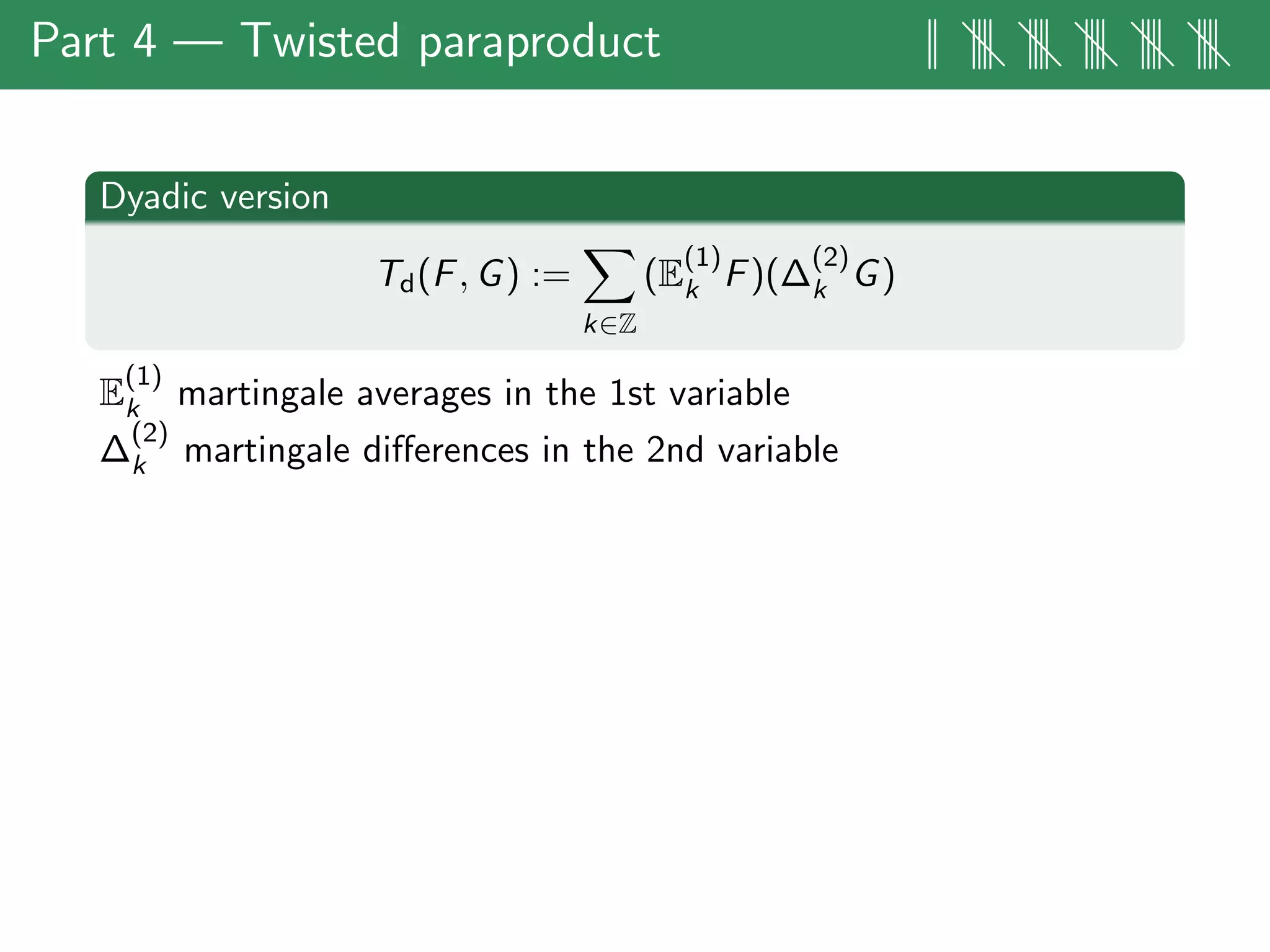
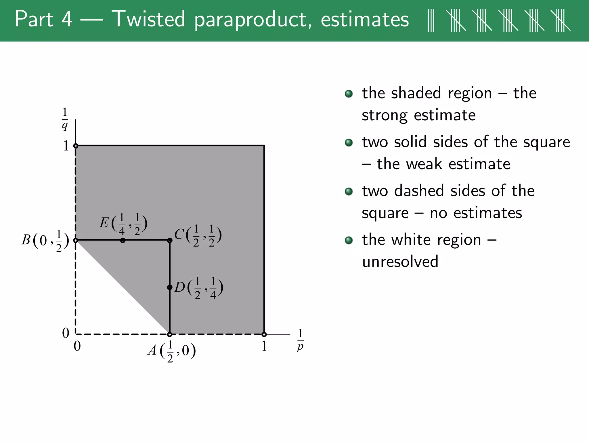
84. Part 4 — Twisted paraproduct || |||| |||| |||| |||| ||||
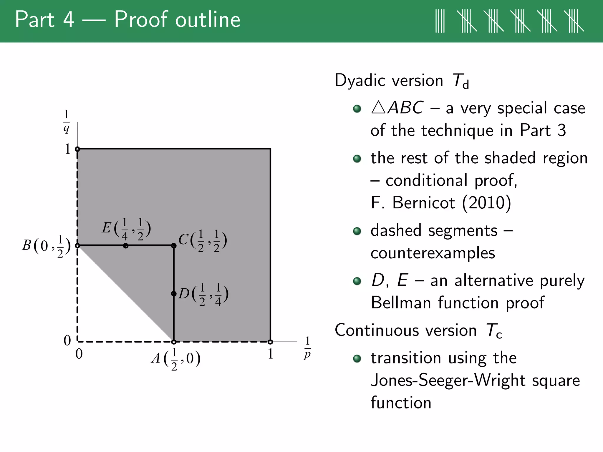
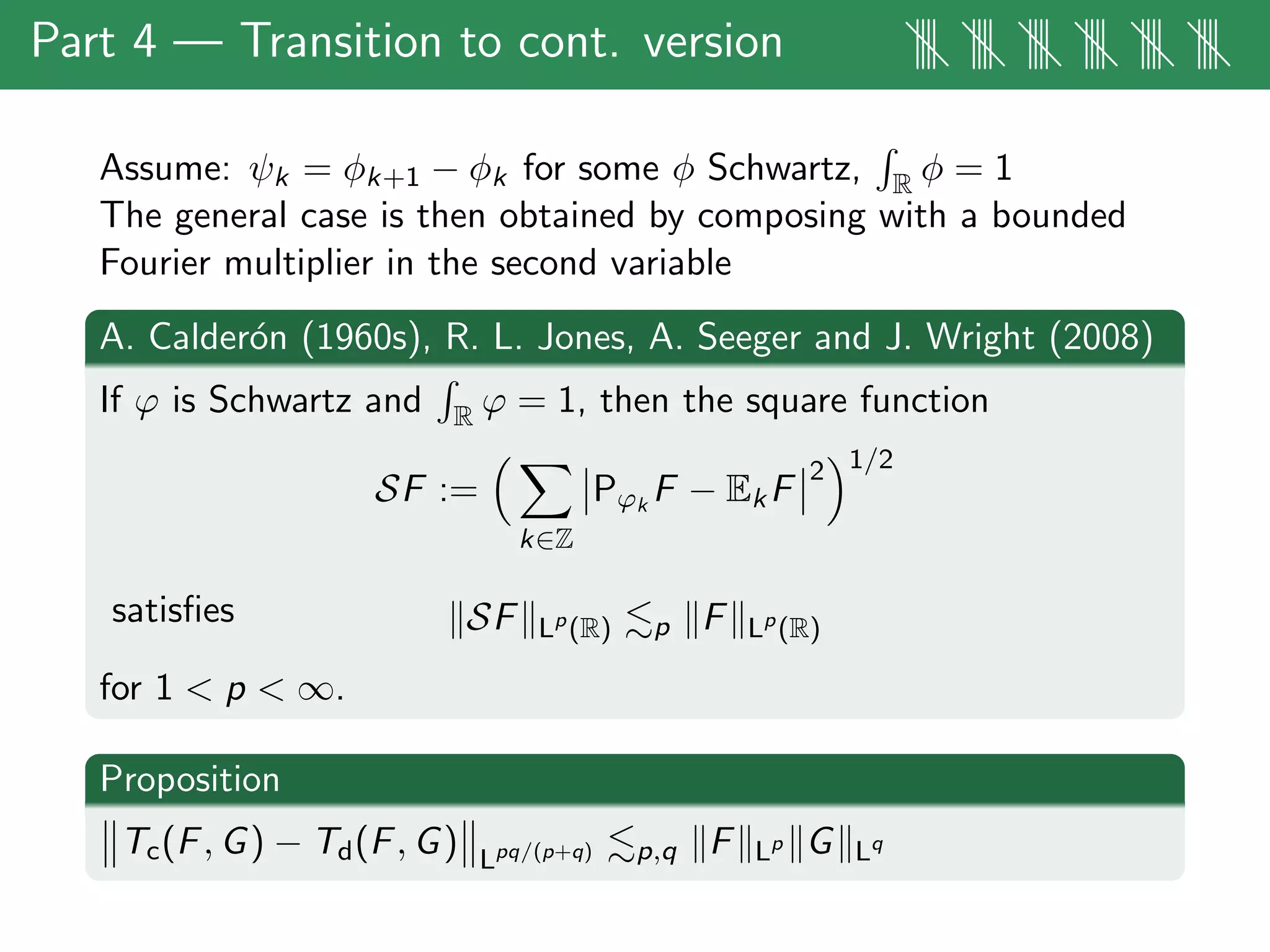
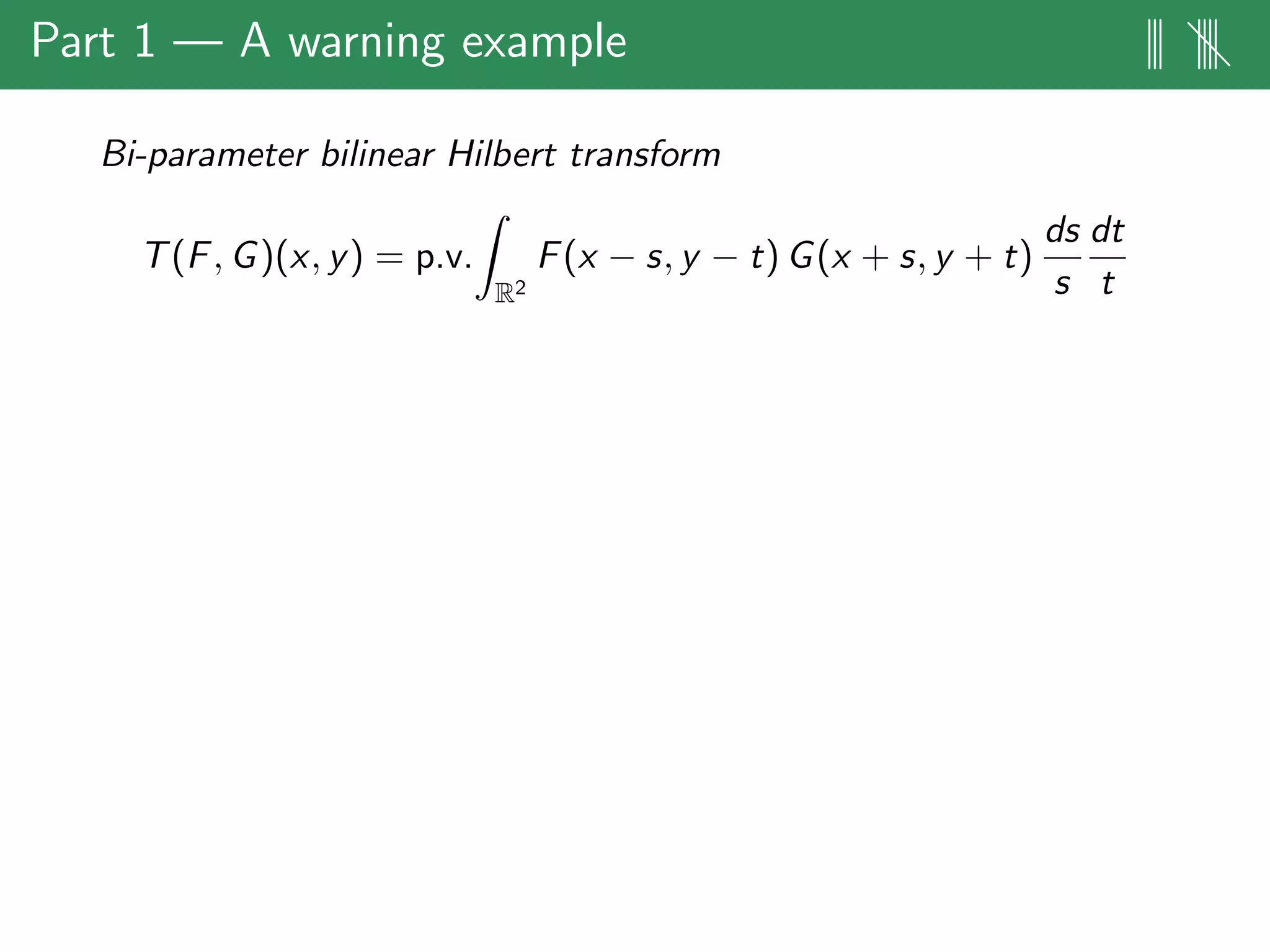
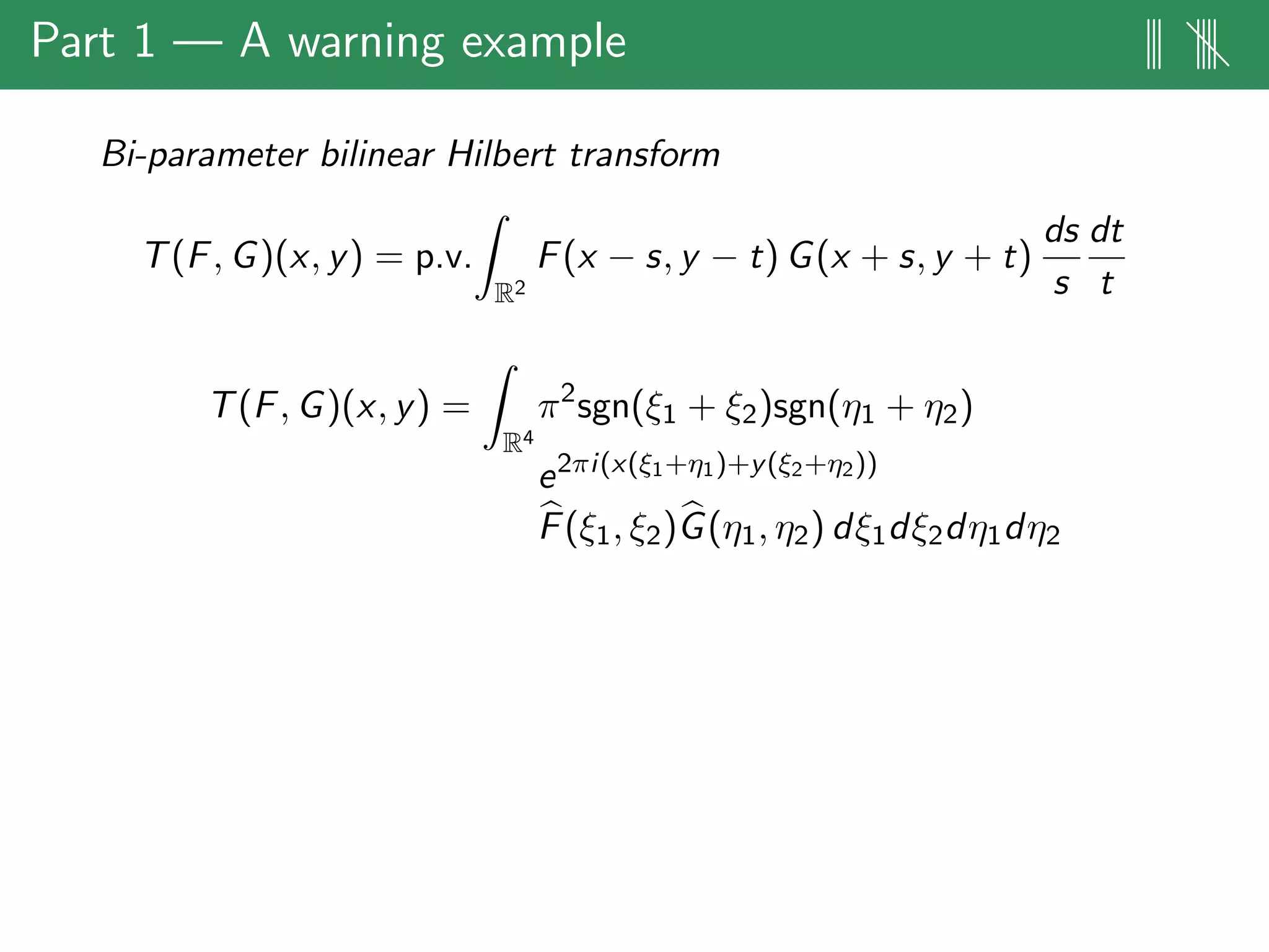
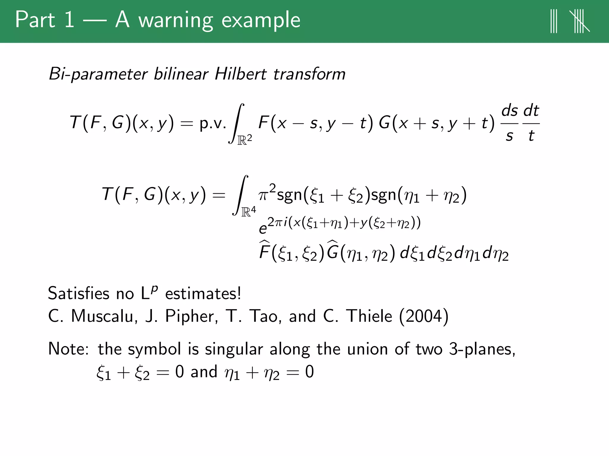
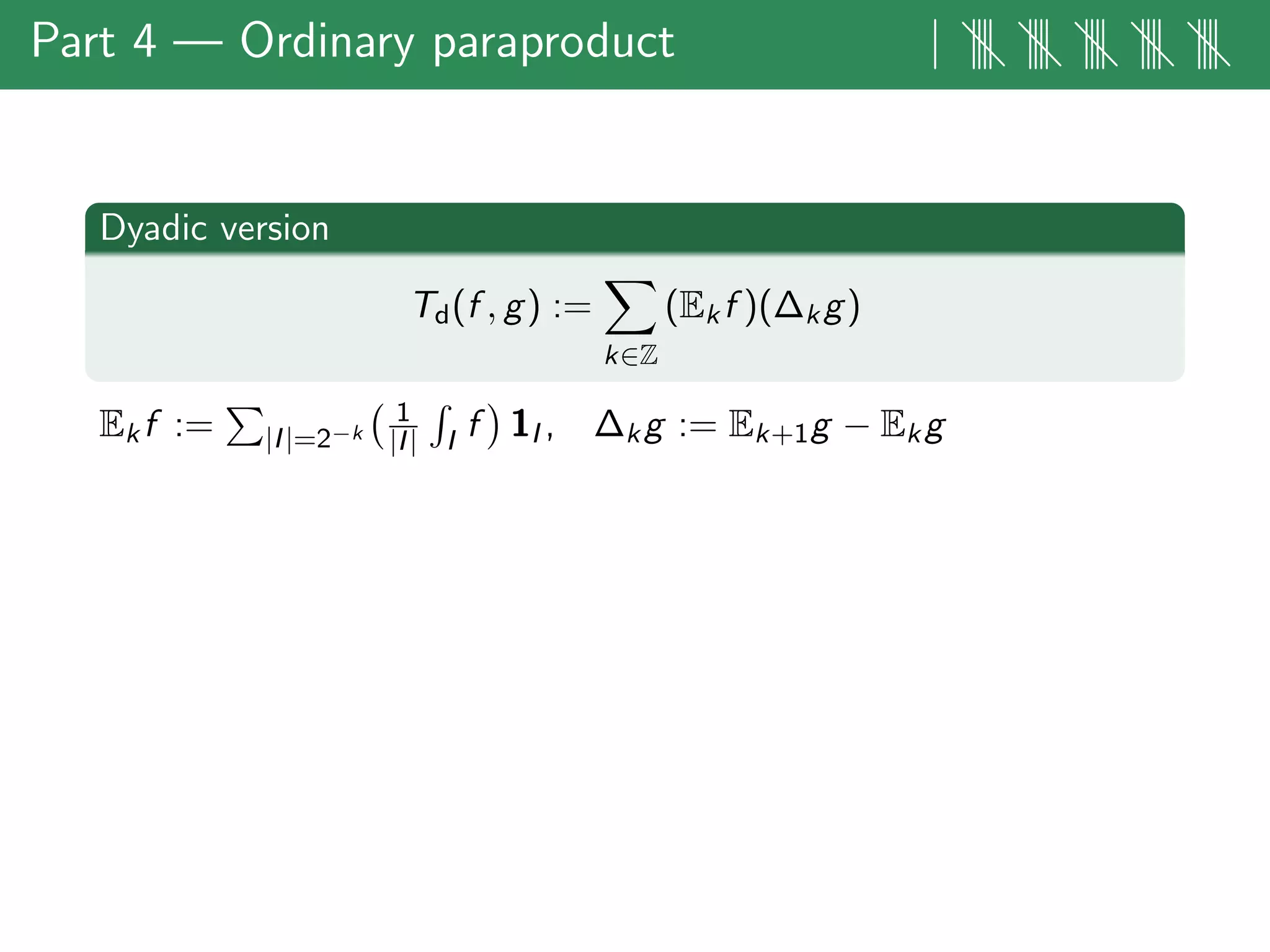
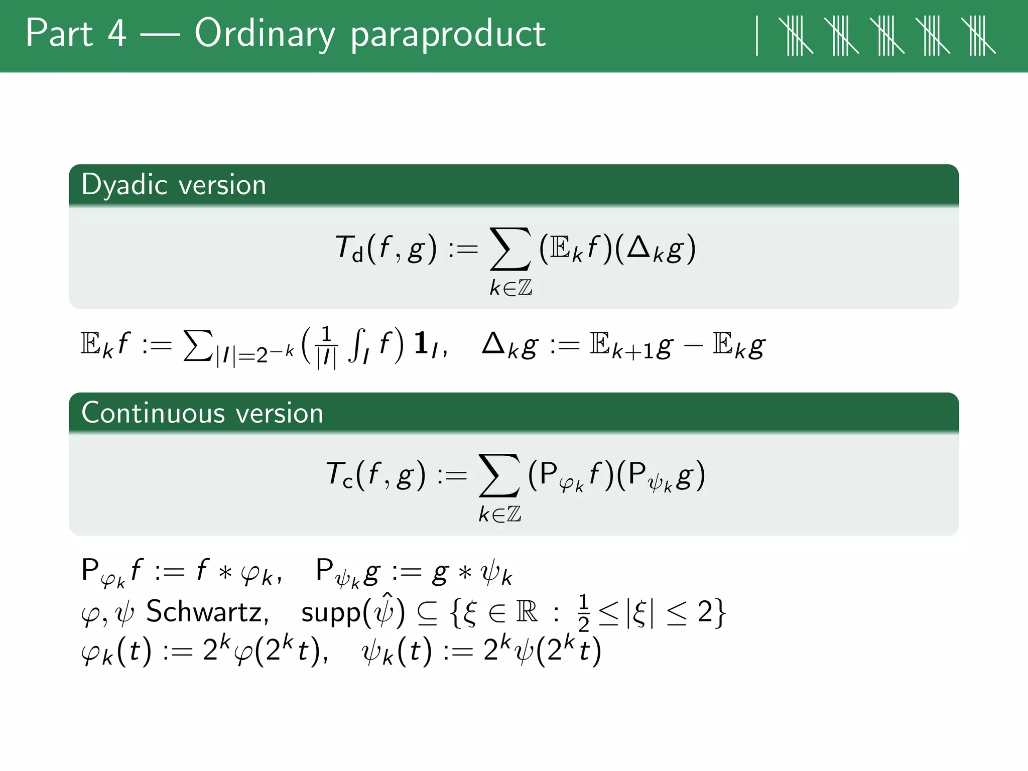
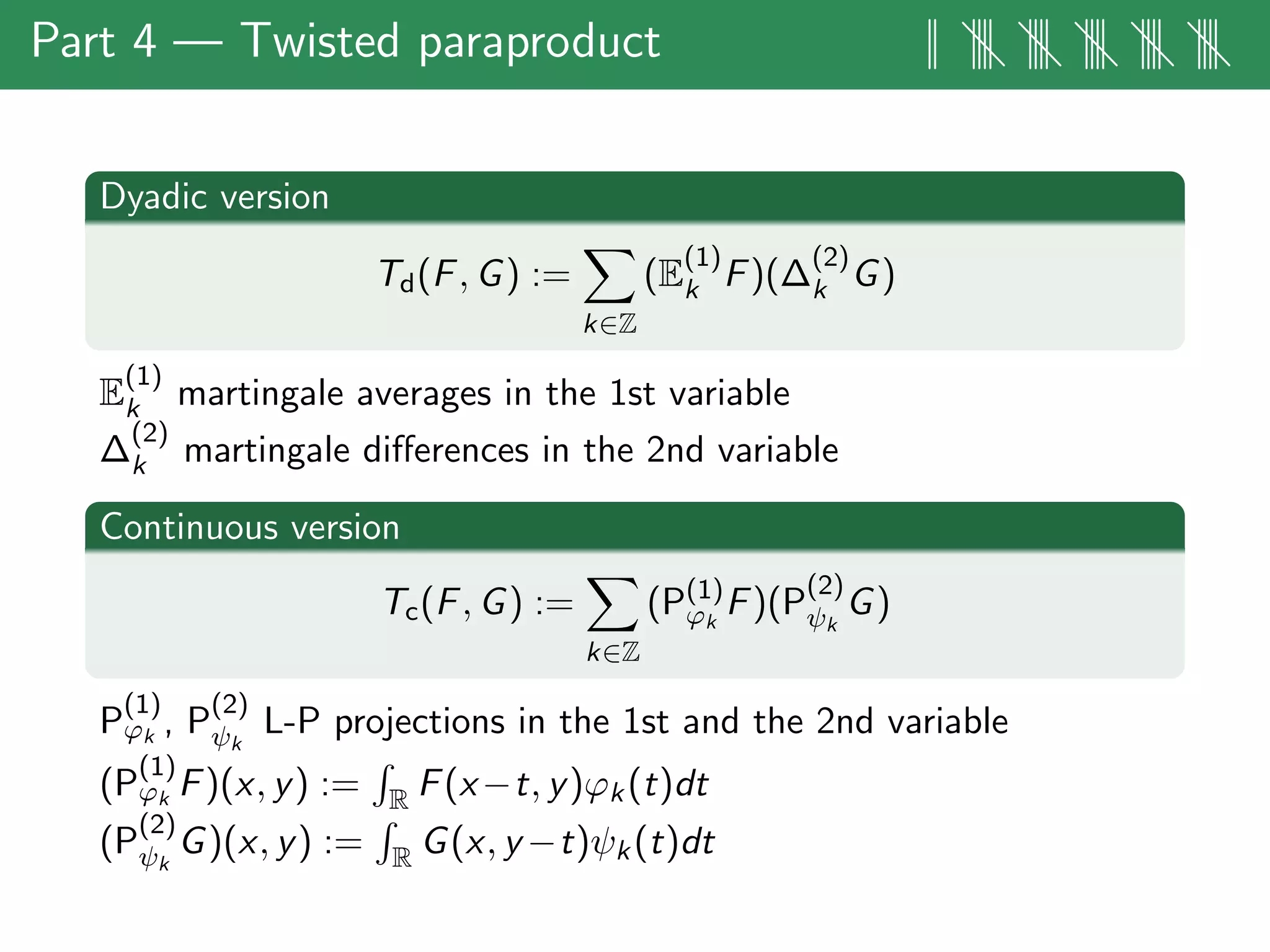
Dyadic version
Td(F, G) :=
k∈Z
(E
(1)
k F)(∆
(2)
k G)
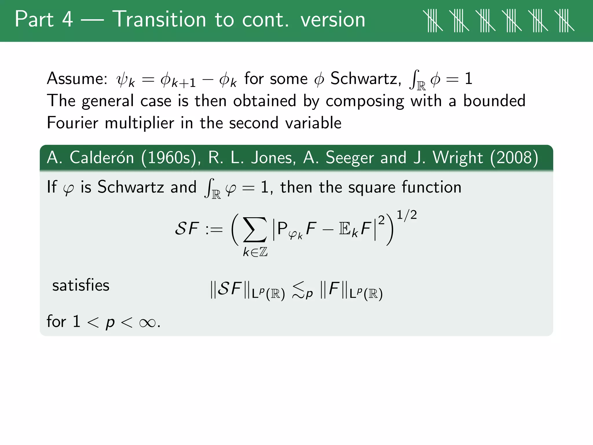
Continuous version
Tc(F, G) :=
k∈Z
(P(1)
ϕk
F)(P
(2)
ψk
G)
Bilinear multipliers from our theorems reduce to these
using cone decomposition of the symbol:
m =
j
m[j]
from the Fourier series
m[j]
(ξ1, η2) =
k∈Z
ϕ
[j]
k (ξ1) ψ
[j]
k (η2)

85. Part 4 — Twisted paraproduct, estimates ||| |||| |||| |||| |||| ||||
B( ), _
2
1 C( )_
2
1 , _
2
1
1
2
_,1
4
_ )(E
D( )_
2
1 ,
0
0,1
2
_ )(A
_
4
1
_1
q
p
1_
1
0
10
the shaded region – the
strong estimate
two solid sides of the square
– the weak estimate
two dashed sides of the
square – no estimates
the white region –
unresolved

86. Part 4 — Proof outline |||| |||| |||| |||| |||| ||||
B( ), _
2
1 C( )_
2
1 , _
2
1
1
2
_,1
4
_ )(E
D( )_
2
1 ,
0
0,1
2
_ )(A
_
4
1
_1
q
p
1_
1
0
10
Dyadic version Td
ABC – a very special case
of the technique in Part 3
the rest of the shaded region
– conditional proof,
F. Bernicot (2010)
dashed segments –
counterexamples
D, E – an alternative purely
Bellman function proof
Continuous version Tc
transition using the
Jones-Seeger-Wright square
function

87. Part 4 — Transition to cont. version |||| |||| |||| |||| |||| ||||
Assume: ψk = φk+1 − φk for some φ Schwartz, R φ = 1
The general case is then obtained by composing with a bounded
Fourier multiplier in the second variable

88. Part 4 — Transition to cont. version |||| |||| |||| |||| |||| ||||
Assume: ψk = φk+1 − φk for some φ Schwartz, R φ = 1
The general case is then obtained by composing with a bounded
Fourier multiplier in the second variable
A. Calder´on (1960s), R. L. Jones, A. Seeger and J. Wright (2008)
If ϕ is Schwartz and R ϕ = 1, then the square function
SF :=
k∈Z
Pϕk
F − EkF
2 1/2
satisfies SF Lp
(R) p F Lp
(R)
for 1 < p < ∞.

89. Part 4 — Transition to cont. version |||| |||| |||| |||| |||| ||||
Assume: ψk = φk+1 − φk for some φ Schwartz, R φ = 1
The general case is then obtained by composing with a bounded
Fourier multiplier in the second variable
A. Calder´on (1960s), R. L. Jones, A. Seeger and J. Wright (2008)
If ϕ is Schwartz and R ϕ = 1, then the square function
SF :=
k∈Z
Pϕk
F − EkF
2 1/2
satisfies SF Lp
(R) p F Lp
(R)
for 1 < p < ∞.
Proposition
Tc(F, G) − Td(F, G) Lpq/(p+q) p,q F Lp G Lq

90. Part 4 — “Entangled” + cont. kernel | |||| |||| |||| |||| |||| ||||
General bipartite graphs G
How to obtain boundedness of
Λ (Fi,j )(i,j)∈E :=
Rm+n
K(x1, . . . , xm, y1, . . . , yn)
(i,j)∈E
Fi,j (xi , yj ) dx1 . . . dxmdy1 . . . dyn
at least for some continuous singular kernels K?

91. Part 4 — “Entangled” + cont. kernel | |||| |||| |||| |||| |||| ||||
General bipartite graphs G
How to obtain boundedness of
Λ (Fi,j )(i,j)∈E :=
Rm+n
K(x1, . . . , xm, y1, . . . , yn)
(i,j)∈E
Fi,j (xi , yj ) dx1 . . . dxmdy1 . . . dyn
at least for some continuous singular kernels K?
We can average “entangled” dyadic operators from Part 3 over
translated, dilated, and rotated dyadic grids
Partial results: One can recover some very special kernels K
Possibly all sufficiently smooth translation-invariant kernels
This is still far from a complete T(1)-type theorem

92. Currently open problems || |||| |||| |||| |||| |||| ||||
Further directions:

93. Currently open problems || |||| |||| |||| |||| |||| ||||
Further directions:
Translating the results to the case of more general continuous
C-Z kernels K
Ultimately obtaining a “real” (i.e. non-dyadic) T(1)-type
theorem

94. Currently open problems || |||| |||| |||| |||| |||| ||||
Further directions:
Translating the results to the case of more general continuous
C-Z kernels K
Ultimately obtaining a “real” (i.e. non-dyadic) T(1)-type
theorem
Forms corresponding to non-bipartite graphs (such as odd
cycles, recall a triangle)

95. Currently open problems || |||| |||| |||| |||| |||| ||||
Further directions:
Translating the results to the case of more general continuous
C-Z kernels K
Ultimately obtaining a “real” (i.e. non-dyadic) T(1)-type
theorem
Forms corresponding to non-bipartite graphs (such as odd
cycles, recall a triangle)
More singular kernels K, like K(x, y, z) = 1
x+y+z

96. Thank you! ||| |||| |||| |||| |||| |||| ||||
Thank you!