Downloaded 12 times


![legall53td.m
function H = legall53td(X)
% Author: Jun Li, more info@ http://goldensectiontransform.org/
%
% function H = legall53td(X,nlevel)
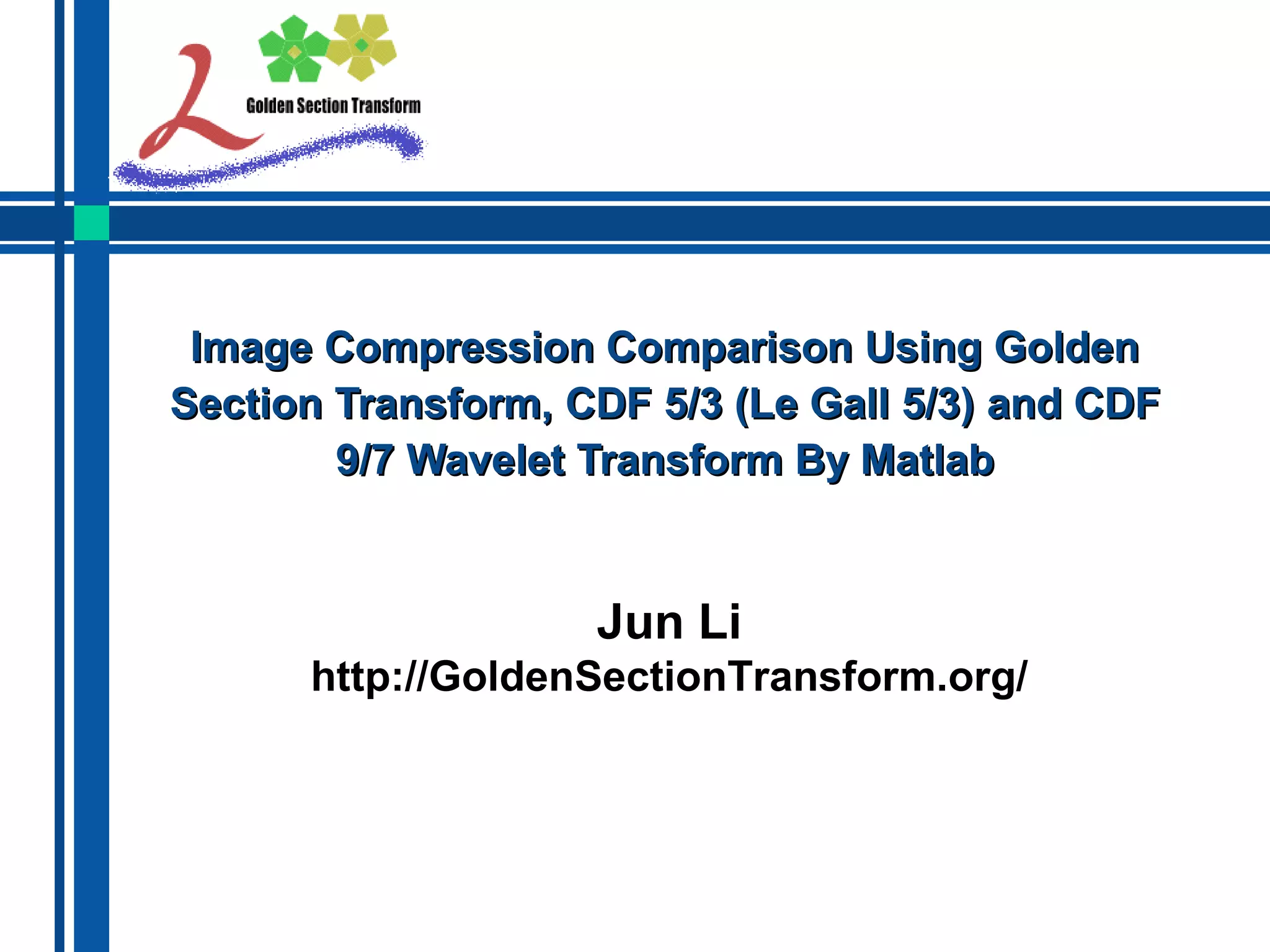
% 3-level 2d LeGall 5/3 wavelet transform of 8*8 image matrix
nlevel = 3; % 3-level transform for each 8*8 image block
[xx,yy] = size(X);
H=X;
for i=1:nlevel
for j=1:xx
[ss,dd] = legall531d(H(j,1:yy)); % row transform
H(j,1:yy) = [ss,dd];
end
for k=1:yy
[ss,dd] = legall531d(H(1:xx,k)'); % column transform
H(1:xx,k) = [ss,dd]';
end
xx = xx/2;
yy = yy/2;
end
%% 1d LeGall 5/3 lifting scheme % symw_ext->...12321...
function [ss,dd] = legall531d(S)
N = length(S);
ga = -1/2;
gb = 1/4;
gc = sqrt(2);
s0 = S(1:2:N-1); % S(1),S(3),S(5),S(7)...
d0 = S(2:2:N); % S(2),S(4),S(6),S(8)...
d1 = d0 + ga*(s0 + [s0(2:N/2) s0(N/2)]);
s1 = s0 + gb*(d1 + [d1(1) d1(1:N/2-1)]);
ss = gc*s1;
dd = d1/gc;](https://image.slidesharecdn.com/image-compression-golden-section-transform-cdf-53-le-gall-53-cdf-97-wavelet-transform-matlab-141003073500-phpapp02/85/Image-Compression-Comparison-Using-Golden-Section-Transform-CDF-5-3-Le-Gall-5-3-and-CDF-9-7-Wavelet-Transform-By-Matlab-10-320.jpg)
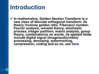
![cdf97td.m function H = cdf97td(X)
% Author: Jun Li, more info@ http://goldensectiontransform.org/
%%
function H = cdf97td(X,nlevel)
% 3-level 2d CDF 9/7 wavelet transform of 8*8 image matrix
nlevel = 3; % 3-level transform for each 8*8 image block
[xx,yy] = size(X);
H=X;
for i=1:nlevel
for j=1:xx
[ss,dd] = cdf971d(H(j,1:yy)); % row transform
H(j,1:yy) = [ss,dd];
end
for k=1:yy
[ss,dd] = cdf971d(H(1:xx,k)'); % column transform
H(1:xx,k) = [ss,dd]';
end
xx = xx/2;
yy = yy/2;
end
%% 1d CDF 9/7 wavelet lifting scheme % symw_ext->...12321...
function [ss,dd] = cdf971d(S)
N = length(S);
fa = -1.586134342;
fb = -0.05298011854;
fc = 0.8829110762;
fd = 0.4435068522;
fz = 1.149604398;
s0 = S(1:2:N-1); % S(1),S(3),S(5),S(7)...
d0 = S(2:2:N); % S(2),S(4),S(6),S(8)...
d1 = d0 + fa*(s0 + [s0(2:N/2) s0(N/2)]);
s1 = s0 + fb*(d1 + [d1(1) d1(1:N/2-1)]);
d2 = d1 + fc*(s1 + [s1(2:N/2) s1(N/2)]);
s2 = s1 + fd*(d2 + [d2(1) d2(1:N/2-1)]);
ss = fz*s2;
dd = d2/fz;](https://image.slidesharecdn.com/image-compression-golden-section-transform-cdf-53-le-gall-53-cdf-97-wavelet-transform-matlab-141003073500-phpapp02/85/Image-Compression-Comparison-Using-Golden-Section-Transform-CDF-5-3-Le-Gall-5-3-and-CDF-9-7-Wavelet-Transform-By-Matlab-11-320.jpg)
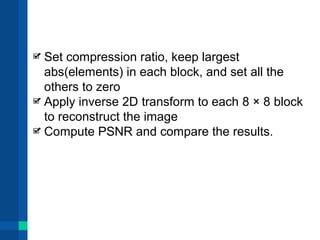
![lgst2d.m
function H = lgst2d(X)
% Author: Jun Li, more info@ http://goldensectiontransform.org/
% function H = lgst2d(X,nlevel)
% 4-level 2d low golden section transform of 8*8 image matrix
nlevel = 4; % 4-level transform for each 8*8 image block
global lj; % only used by function lgst1d(S) below.
global FBL; % only used by function lgst1d(S) below.
[xx,yy] = size(X);
ind = floor(log(xx*sqrt(5)+1/2)/log((sqrt(5)+1)/2)); % determine index
FBL = filter(1,[1 -1 -1],[1 zeros(1,ind-1)]);
% FBL = Fibonacci sequence -> [1 1 2 3 5 8...];
H=X;
for lj=1:nlevel
for j=1:xx
[ss,dd] = lgst1d(H(j,1:yy)); % row transform
H(j,1:yy) = [ss,dd];
end
for k=1:yy
[ss,dd] = lgst1d(H(1:xx,k)'); % column transform
H(1:xx,k) = [ss,dd]';
end
xx = FBL(end-lj); % round((sqrt(5)-1)/2*xx); 8*8 block: xx=8->5->3->2
yy = FBL(end-lj); % round((sqrt(5)-1)/2*yy); 8*8 block: yy=8->5->3->2
end
%% 1d low golden section transform
function [ss,dd] = lgst1d(S)
global lj;
global FBL;
index = 0;
h = 1;
lform = lword(length(S));
for i=1:length(lform)
index = index + lform(i);
if lform(i) == 1
ss(i) = S(index);
else % lform(i) == 2
ss(i) = (sqrt(FBL(lj))*S(index-1)+sqrt(FBL(lj+1))*S(index))/sqrt(FBL(lj+2));
dd(h) = (sqrt(FBL(lj+1))*S(index-1)-sqrt(FBL(lj))*S(index))/sqrt(FBL(lj+2));
h = h+1;
end
end](https://image.slidesharecdn.com/image-compression-golden-section-transform-cdf-53-le-gall-53-cdf-97-wavelet-transform-matlab-141003073500-phpapp02/85/Image-Compression-Comparison-Using-Golden-Section-Transform-CDF-5-3-Le-Gall-5-3-and-CDF-9-7-Wavelet-Transform-By-Matlab-12-320.jpg)
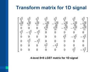
![lword.m
function lform = lword(n)
% Author: Jun Li, more info@ http://goldensectiontransform.org/
% Type-L golden section decomposion of fibonacci number n,
% e.g. lword(8) = [1 2 2 1 2];
if n == 1
lform = [1];
elseif n == 2
lform = [2];
else
next = round((sqrt(5)-1)/2*n);
lform = [lword(n-next),lword(next)];
end](https://image.slidesharecdn.com/image-compression-golden-section-transform-cdf-53-le-gall-53-cdf-97-wavelet-transform-matlab-141003073500-phpapp02/85/Image-Compression-Comparison-Using-Golden-Section-Transform-CDF-5-3-Le-Gall-5-3-and-CDF-9-7-Wavelet-Transform-By-Matlab-13-320.jpg)
![hgst2d.m
function H = hgst2d(X)
% Author: Jun Li, more info@ http://goldensectiontransform.org/
% function H = hgst2d(X,nlevel)
% 2-level 2d high golden section transform of 8*8 image matrix
nlevel = 2; % 2-level transform for each 8*8 image block
global hj; % only used by function hgst1d(S) below.
global FBH; % only used by function hgst1d(S) below.
[xx,yy] = size(X);
ind = floor(log(xx*sqrt(5)+1/2)/log((sqrt(5)+1)/2)); % determine index
FBH = filter(1,[1 -1 -1],[1 zeros(1,ind-1)]);
% FBH = Fibonacci sequence -> [1 1 2 3 5 8...];
H=X;
for hj=1:nlevel
for j=1:xx
[ss,dd] = hgst1d(H(j,1:yy)); % row transform
H(j,1:yy) = [ss,dd];
end
for k=1:yy
[ss,dd] = hgst1d(H(1:xx,k)'); % column transform
H(1:xx,k) = [ss,dd]';
end
xx = FBH(end-2*hj); % round((3-sqrt(5))/2*xx); 8*8 block: xx=8->3
yy = FBH(end-2*hj); % round((3-sqrt(5))/2*yy); 8*8 block: yy=8->3
end
%% 1d high golden section transform
function [ss,dd] = hgst1d(S)
global hj;
global FBH;
index = 0;
g = 1;
h = 1;
hform = hword(length(S));
for i=1:length(hform)
index = index + hform(i);
if hform(i) == 2
ss(i) = (sqrt(FBH(2*hj-1))*S(index-1)+sqrt(FBH(2*hj))*S(index))/sqrt(FBH(2*hj+1));
dd(2*i-g) = (sqrt(FBH(2*hj))*S(index-1)-sqrt(FBH(2*hj-1))*S(index))/sqrt(FBH(2*hj+1));
g = g+1;
else % hform(i) == 3
ss(i) = (sqrt(FBH(2*hj))*S(index-2)+sqrt(FBH(2*hj-1))*S(index-1)+sqrt(FBH(2*hj))*S(index))/sqrt(FBH(2*hj+2));
dd(i+h-1) = (sqrt(FBH(2*hj-1))*S(index-2)-2*sqrt(FBH(2*hj))*S(index-1)+sqrt(FBH(2*hj-1))*S(index))/sqrt(2*FBH(2*hj+2));
dd(i+h) = (S(index-2)-S(index))/sqrt(2);
h = h+1;
end
end](https://image.slidesharecdn.com/image-compression-golden-section-transform-cdf-53-le-gall-53-cdf-97-wavelet-transform-matlab-141003073500-phpapp02/85/Image-Compression-Comparison-Using-Golden-Section-Transform-CDF-5-3-Le-Gall-5-3-and-CDF-9-7-Wavelet-Transform-By-Matlab-14-320.jpg)
![hword.m
function hform = hword(n)
% Author: Jun Li, more info@ http://goldensectiontransform.org/
% Type-H golden section decomposion of fibonacci number n,
% e.g. hword(8) = [3 2 3];
if n == 2
hform = [2];
elseif n == 3
hform = [3];
else
next = round((sqrt(5)-1)/2*n);
hform = [hword(n-next),hword(next)];
end](https://image.slidesharecdn.com/image-compression-golden-section-transform-cdf-53-le-gall-53-cdf-97-wavelet-transform-matlab-141003073500-phpapp02/85/Image-Compression-Comparison-Using-Golden-Section-Transform-CDF-5-3-Le-Gall-5-3-and-CDF-9-7-Wavelet-Transform-By-Matlab-15-320.jpg)
![keep.m
function X = keep(X)
% keep the largest abs(elements) of X,
% global RATIO set in gstdemo.m is in [0,1].
global RATIO;
N = floor(prod(size(X))*RATIO);
[MM,i] = sort(abs(X(:)));
X(i(1:end-N)) = 0;](https://image.slidesharecdn.com/image-compression-golden-section-transform-cdf-53-le-gall-53-cdf-97-wavelet-transform-matlab-141003073500-phpapp02/85/Image-Compression-Comparison-Using-Golden-Section-Transform-CDF-5-3-Le-Gall-5-3-and-CDF-9-7-Wavelet-Transform-By-Matlab-16-320.jpg)
![psnr.m
function [MSE,PSNR] = psnr(X,Y)
% Compute MSE and PSNR.
MSE = sum((X(:)-Y(:)).^2)/prod(size(X));
if MSE == 0
PSNR = Inf;
else
PSNR = 10*log10(255^2/MSE);
end](https://image.slidesharecdn.com/image-compression-golden-section-transform-cdf-53-le-gall-53-cdf-97-wavelet-transform-matlab-141003073500-phpapp02/85/Image-Compression-Comparison-Using-Golden-Section-Transform-CDF-5-3-Le-Gall-5-3-and-CDF-9-7-Wavelet-Transform-By-Matlab-17-320.jpg)
![References
[1] Jun. Li (2007). "Golden Section Method Used in Digital Image Multi-resolution Analysis".
Application Research of Computers (in zh-cn) 24 (Suppl.): 1880–1882. ISSN 1001-
3695;CN 51-1196/TP
[2] I. Daubechies and W. Sweldens, "Factoring wavelet transforms into lifting schemes," J.
Fourier Anal. Appl., vol. 4, no. 3, pp. 247-269, 1998.
[3] Ingrid Daubechies. 1992. Ten Lectures on Wavelets. Soc. for Industrial and Applied
Math., Philadelphia, PA, USA.
[4] Sun, Y.K.(2005). Wavelet Analysis and Its Applications. China Machine Press. ISBN
7111158768
[5] Jin, J.F.(2004). Visual C++ Wavelet Transform Technology and Engineering Practice.
Posts & Telecommunications Press. ISBN 7115119597
[6] He, B.;Ma, T.Y.(2002). Visual C++ Digital Image Processing. Posts & Telecommunications
Press. ISBN 7115109559
[7] V. Britanak, P. Yip, K. R. Rao, 2007 Discrete Cosine and Sine Transform, General
properties, Fast Algorithm and Integer Approximations" Academic Press
[8] K. R. Rao and P. Yip, Discrete Cosine Transform: Algorithms, Advantages, Applications,
Academic Press, Boston, 1990.
[9] J. Nilsson, On the entropy of random Fibonacci words, arXiv:1001.3513.
[10] J. Nilsson, On the entropy of a family of random substitutions, Monatsh. Math. 168
(2012) 563–577. arXiv:1103.4777.](https://image.slidesharecdn.com/image-compression-golden-section-transform-cdf-53-le-gall-53-cdf-97-wavelet-transform-matlab-141003073500-phpapp02/85/Image-Compression-Comparison-Using-Golden-Section-Transform-CDF-5-3-Le-Gall-5-3-and-CDF-9-7-Wavelet-Transform-By-Matlab-22-320.jpg)
![[11] J. Nilsson, On the entropy of a two step random Fibonacci substitution, Entropy 15
(2013) 3312—3324; arXiv:1303.2526.
[12] Wai-Fong Chuan, Fang-Yi Liao, Hui-Ling Ho, and Fei Yu. 2012. Fibonacci word patterns
in two-way infinite Fibonacci words. Theor. Comput. Sci. 437 (June 2012), 69-81.
DOI=10.1016/j.tcs.2012.02.020 http://dx.doi.org/10.1016/j.tcs.2012.02.020
[13] Julien Cassaigne (2008). On extremal properties of the Fibonacci word. RAIRO -
Theoretical Informatics and Applications, 42, pp 701-715. doi:10.1051/ita:2008003.
[14] Wojciech Rytter, The structure of subword graphs and suffix trees of Fibonacci words,
Theoretical Computer Science, Volume 363, Issue 2, 28 October 2006, Pages 211-223,
ISSN 0304-3975, http://dx.doi.org/10.1016/j.tcs.2006.07.025.
[15] Alex Vinokur, Fibonacci connection between Huffman codes and Wythoff array,
arXiv:cs/0410013v2
[16] Vinokur A.B., Huffman trees and Fibonacci numbers. Kibernetika Issue 6 (1986) 9-12 (in
Russian), English translation in Cybernetics 22 Issue 6 (1986) 692–696;
http://springerlink.metapress.com/link.asp?ID=W32X70520K8JJ617
[17] L. Colussi, Fastest Pattern Matching in Strings, Journal of Algorithms, Volume 16, Issue
2, March 1994, Pages 163-189, ISSN 0196-6774,
http://dx.doi.org/10.1006/jagm.1994.1008.
[18] Ron Lifshitz, The square Fibonacci tiling, Journal of Alloys and Compounds, Volume
342, Issues 1–2, 14 August 2002, Pages 186-190, ISSN 0925-8388,
http://dx.doi.org/10.1016/S0925-8388(02)00169-X.
[19] C. Godr`eche, J. M. Luck, Quasiperiodicity and randomness in tilings of the plane,
Journal of Statistical Physics, Volume 55, Issue 1–2, pp. 1–28.
[20] S. Even-Dar Mandel and R. Lifshitz. Electronic energy spectra and wave functions on
the square Fibonacci tiling. Philosophical Magazine, 86:759-764, 2006.](https://image.slidesharecdn.com/image-compression-golden-section-transform-cdf-53-le-gall-53-cdf-97-wavelet-transform-matlab-141003073500-phpapp02/85/Image-Compression-Comparison-Using-Golden-Section-Transform-CDF-5-3-Le-Gall-5-3-and-CDF-9-7-Wavelet-Transform-By-Matlab-23-320.jpg)
![[21] S. Goedecker. 1997. Fast Radix 2, 3, 4, and 5 Kernels for Fast Fourier Transformations
on Computers with Overlapping Multiply--Add Instructions. SIAM J. Sci. Comput. 18, 6
(November 1997), 1605-1611. DOI=10.1137/S1064827595281940
http://dx.doi.org/10.1137/S1064827595281940
[22] Bashar, S.K., "An efficient approach to the computation of fast fourier transform(FFT)
by Radix-3 algorithm," Informatics, Electronics & Vision (ICIEV), 2013 International
Conference on , vol., no., pp.1,5, 17-18 May 2013
[23] Lofgren, J.; Nilsson, P., "On hardware implementation of radix 3 and radix 5 FFT
kernels for LTE systems," NORCHIP, 2011 , vol., no., pp.1,4, 14-15 Nov. 2011
[24] Prakash, S.; Rao, V.V., "A new radix-6 FFT algorithm," Acoustics, Speech and Signal
Processing, IEEE Transactions on , vol.29, no.4, pp.939,941, Aug 1981
[25] Suzuki, Y.; Toshio Sone; Kido, K., "A new FFT algorithm of radix 3,6, and 12,"
Acoustics, Speech and Signal Processing, IEEE Transactions on , vol.34, no.2,
pp.380,383, Apr 1986
[26] Dubois, E.; Venetsanopoulos, A., "A new algorithm for the radix-3 FFT," Acoustics,
Speech and Signal Processing, IEEE Transactions on , vol.26, no.3, pp.222,225, Jun
1978
[27] S. Goedecker. 1997. Fast Radix 2, 3, 4, and 5 Kernels for Fast Fourier Transformations
on Computers with Overlapping Multiply--Add Instructions. SIAM J. Sci. Comput. 18, 6
(November 1997), 1605-1611. DOI=10.1137/S1064827595281940
http://dx.doi.org/10.1137/S1064827595281940
[28] Huazhong Shu; XuDong Bao; Toumoulin, C.; Limin Luo, "Radix-3 Algorithm for the Fast
Computation of Forward and Inverse MDCT," Signal Processing Letters, IEEE , vol.14,
no.2, pp.93,96, Feb. 2007
[29] Guoan Bi; Yu, L.W., "DCT algorithms for composite sequence lengths," Signal
Processing, IEEE Transactions on , vol.46, no.3, pp.554,562, Mar 1998
[30] Yuk-Hee Chan; Wan-Chi Siu,, "Fast radix-3/6 algorithms for the realization of the
discrete cosine transform," Circuits and Systems, 1992. ISCAS '92. Proceedings., 1992
IEEE International Symposium on , vol.1, no., pp.153,156 vol.1, 10-13 May 1992](https://image.slidesharecdn.com/image-compression-golden-section-transform-cdf-53-le-gall-53-cdf-97-wavelet-transform-matlab-141003073500-phpapp02/85/Image-Compression-Comparison-Using-Golden-Section-Transform-CDF-5-3-Le-Gall-5-3-and-CDF-9-7-Wavelet-Transform-By-Matlab-24-320.jpg)
![[31] Yiquan Wu; Zhaoda Zhu, "New radix-3 fast algorithm for the discrete cosine transform,"
Aerospace and Electronics Conference, 1993. NAECON 1993., Proceedings of the IEEE
1993 National , vol., no., pp.86,89 vol.1, 24-28 May 1993
[32] Huazhong Shu; XuDong Bao; Toumoulin, C.; Limin Luo, "Radix-3 Algorithm for the Fast
Computation of Forward and Inverse MDCT," Signal Processing Letters, IEEE , vol.14,
no.2, pp.93,96, Feb. 2007
[33] Yuk-Hee Chan; Wan-Chi Siu,, "Mixed-radix discrete cosine transform," Signal
Processing, IEEE Transactions on , vol.41, no.11, pp.3157,3161, Nov 1993
[34] Yuk-Hee Chan; Wan-Chi Siu,, "Fast radix-3/6 algorithms for the realization of the
discrete cosine transform," Circuits and Systems, 1992. ISCAS '92. Proceedings., 1992
IEEE International Symposium on , vol.1, no., pp.153,156 vol.1, 10-13 May 1992
[35] Jiasong Wu; Lu Wang; Senhadji, L.; Huazhong Shu, "Improved radix-3 decimation-in-frequency
algorithm for the fast computation of forward and inverse MDCT," Audio
Language and Image Processing (ICALIP), 2010 International Conference on , vol., no.,
pp.694,699, 23-25 Nov. 2010
[36] Sanchez, V.; Garcia, P.; Peinado, AM.; Segura, J.C.; Rubio, AJ., "Diagonalizing
properties of the discrete cosine transforms," Signal Processing, IEEE Transactions
on , vol.43, no.11, pp.2631,2641, Nov 1995
[37] Lun, Daniel Pak-Kong; Wan-Chi Siu,, "Fast radix-3/9 discrete Hartley transform," Signal
Processing, IEEE Transactions on , vol.41, no.7, pp.2494,2499, Jul 1993
[38] Huazhong Shu; Jiasong Wu; Chunfeng Yang; Senhadji, L., "Fast Radix-3 Algorithm for
the Generalized Discrete Hartley Transform of Type II," Signal Processing Letters, IEEE ,
vol.19, no.6, pp.348,351, June 2012
[39] Prabhu, K.M.M.; Nagesh, A., "New radix-3 and 6 decimation-in-frequency fast Hartley
transform algorithms," Electrical and Computer Engineering, Canadian Journal of ,
vol.18, no.2, pp.65,69, April 1993
[40] Sorensen, H.V.; Jones, D.L.; Burrus, C.S.; Heideman, M., "On computing the discrete
Hartley transform," Acoustics, Speech and Signal Processing, IEEE Transactions on ,
vol.33, no.5, pp.1231,1238, Oct 1985](https://image.slidesharecdn.com/image-compression-golden-section-transform-cdf-53-le-gall-53-cdf-97-wavelet-transform-matlab-141003073500-phpapp02/85/Image-Compression-Comparison-Using-Golden-Section-Transform-CDF-5-3-Le-Gall-5-3-and-CDF-9-7-Wavelet-Transform-By-Matlab-25-320.jpg)
![[41] Wu, J.S.; Shu, H.Z.; Senhadji, L.; Luo, L.M., "Radix-3-3 Algorithm for The 2-D Discrete
Hartley Transform," Circuits and Systems II: Express Briefs, IEEE Transactions on ,
vol.55, no.6, pp.566,570, June 2008
[42] Prabhu, K. M M, "An efficient radix-3 FHT algorithm," Digital Signal Processing
Proceedings, 1997. DSP 97., 1997 13th International Conference on , vol.1, no.,
pp.349,351 vol.1, 2-4 Jul 1997
[43] Zhao, Z.-J., "In-place radix-3 fast Hartley transform algorithm," Electronics Letters ,
vol.28, no.3, pp.319,321, 30 Jan. 1992
[44] Anupindi, N.; Narayanan, S.B.; Prabhu, K.M.M., "New radix-3 FHT algorithm,"
Electronics Letters , vol.26, no.18, pp.1537,1538, 30 Aug. 1990
[45] Yiquan Wu; Zhaoda Zhu, "A new radix-3 fast algorithm for computing the DST-II,"
Aerospace and Electronics Conference, 1995. NAECON 1995., Proceedings of the IEEE
1995 National , vol.1, no., pp.324,327 vol.1, 22-26 May 1995](https://image.slidesharecdn.com/image-compression-golden-section-transform-cdf-53-le-gall-53-cdf-97-wavelet-transform-matlab-141003073500-phpapp02/85/Image-Compression-Comparison-Using-Golden-Section-Transform-CDF-5-3-Le-Gall-5-3-and-CDF-9-7-Wavelet-Transform-By-Matlab-26-320.jpg)

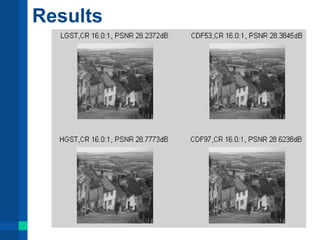
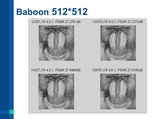
The document discusses various image compression techniques using Golden Section Transforms and Wavelet Transforms, specifically implemented in MATLAB. It highlights the methodology of compressing images by dividing them into blocks, applying transforms, and analyzing performance metrics like PSNR. Additionally, it provides MATLAB code for different transforms and references related literature in the field of digital signal processing.


![Getting Started with Apache Spark: Big Data Made Simple [Free Meetup]](https://cdn.slidesharecdn.com/ss_thumbnails/apachesparkgettingstarted-260203175547-8361bcc3-thumbnail.jpg?width=640&height=640&fit=bounds)


