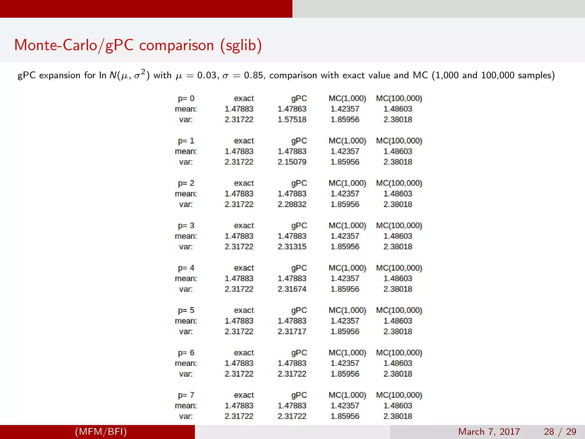
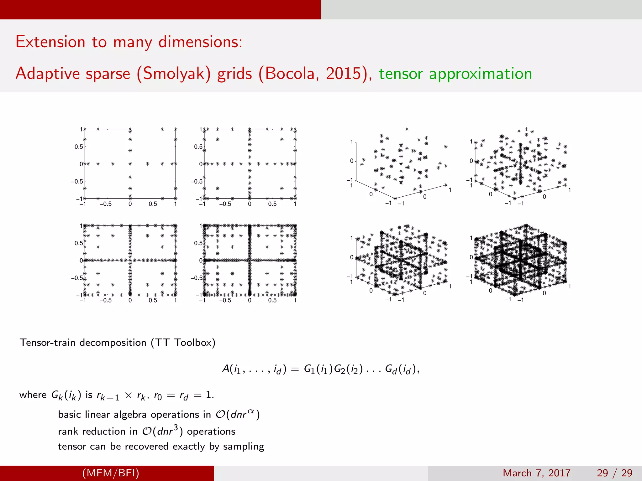
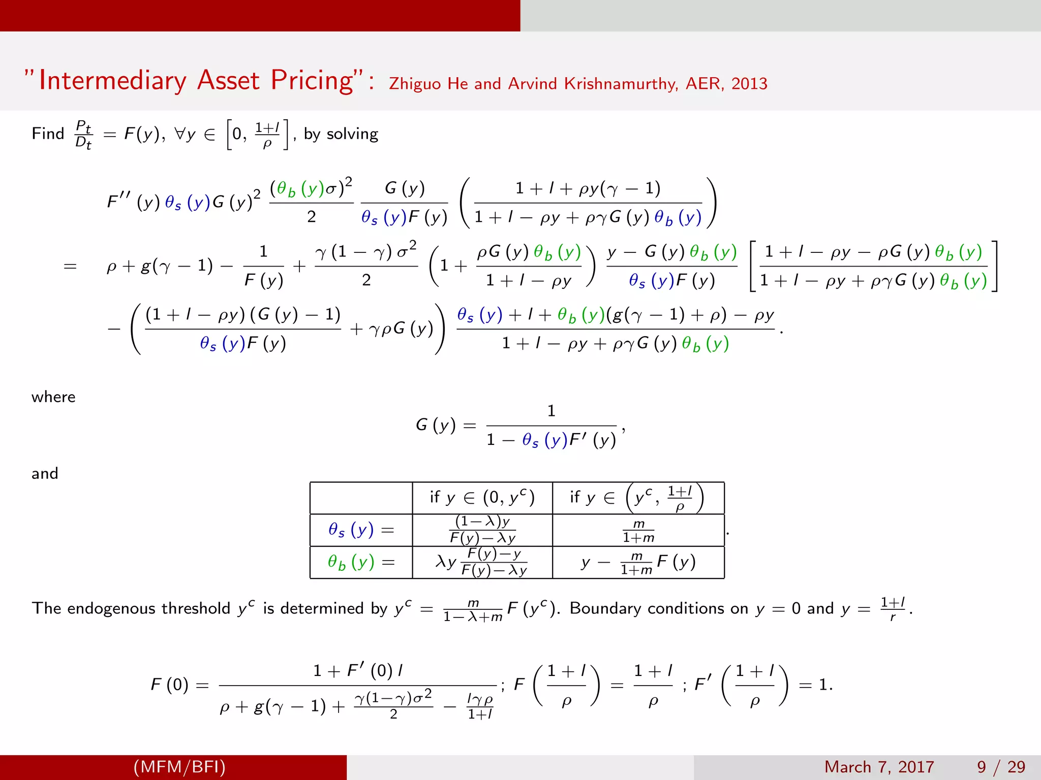
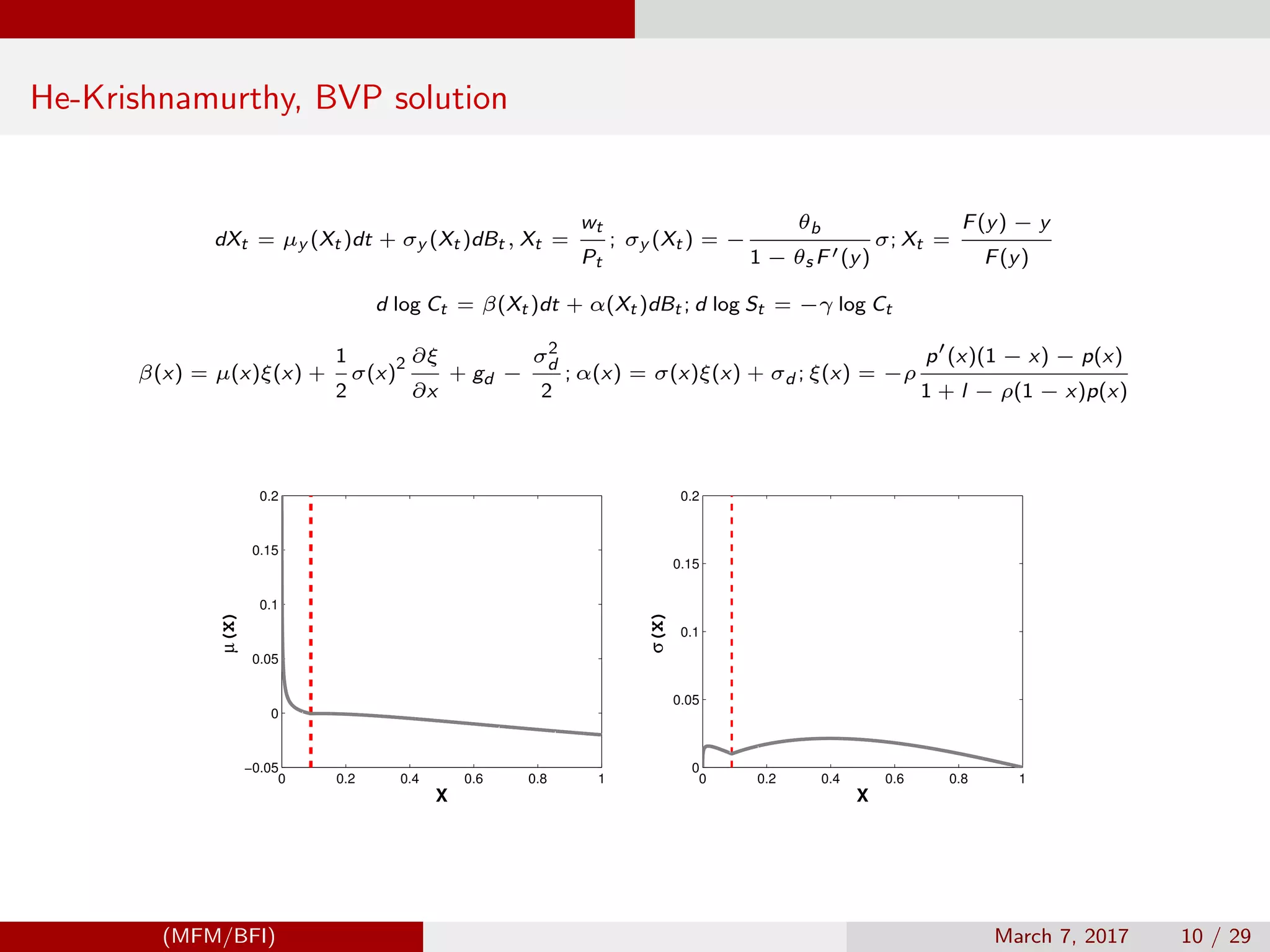
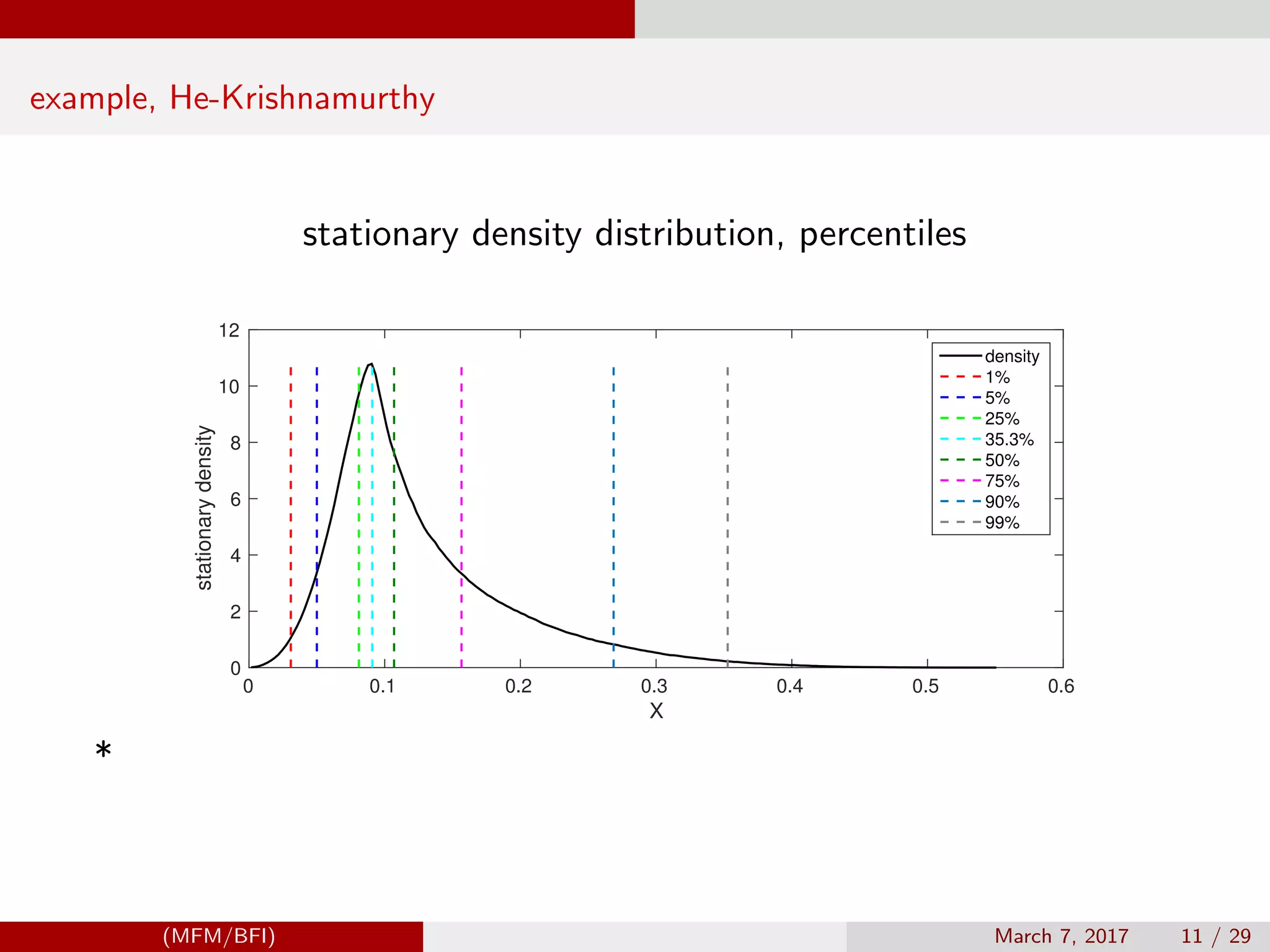
The document discusses computational tools and techniques for numerical macro-financial modeling, focusing on various numerical building blocks such as spectral approximation, adaptive quadratures, and stochastic processes. It presents models and methods for asset pricing and shock elasticities, comparing different computational strategies and their efficacy. Additionally, it includes specific modeling examples and equations relevant to intermediary asset pricing and elasticity calculations.

1. Computational Tools and Techniques
for Numerical Macro-Financial Modeling
Victor V. Zhorin
MFM/BFI
March 7, 2017
(MFM/BFI) March 7, 2017 1 / 29

2. Numerical Building Blocks
Spectral approximation technology (chebfun):
numerical computation in Chebyshev functions
piece-wise smooth functions
breakpoints detection
rootfinding
functions with singularities
fast adaptive quadratures
continuous QR, SVD, least-squares
linear operators
solution of linear and non-linear ODE
Fr´echet derivatives via automatic differentiation
PDEs in one space variable plus time
Stochastic processes:
(quazi) Monte-Carlo simulations, Polynomial Expansion (gPC), finite-differences (FD)
non-linear IRF
Boroviˇcka-Hansen-Sc[heinkman shock-exposure and shock-price elasticities
Malliavin derivatives
Many states:
Dimensionality Curse Cure
low-rank tensor decomposition
sparse Smolyak grids
(MFM/BFI) March 7, 2017 2 / 29

3. Numerical Building Blocks (cont.)
non-
linear
model
shocks
(q)MC
gPC
FD
many
states
low
rank TT
sparse
grids
spectral
tech
non-
linear
ODE
BVP
roots,
Pad´e
, ∂(n)
∂x(n)
MFM
(MFM/BFI) March 7, 2017 3 / 29

4. Horse race: methods and models
models
He-Krishnamurthy, ”Intermediary Asset Pricing”
Klimenko-Pfeil-Rochet-DeNicolo, ”Aggregate Bank Capital and Credit Dynamics”
Brunnermeier-Sannikov, ”A Macroeconomic Model with a Financial Sector”
Basak-Cuoco, ”An Equilibrium Model with Restricted Stock Market Participation”
Di Tella, ”Uncertainty Shocks and Balance Sheet Recessions”
methods
spectral technology vs discrete grids
Monte-Carlo simulations (MC) vs Polynomial Expansion (gPC) vs finite-differences SPDE (FD)
Smolyak sparse grids vs tensor decomposition
criteria
elegance: clean primitives, libraries, ease of mathematical concepts expression in code
speed: feasibility, ready prototypes, LEGO blocks; precision: numerical tests of speed vs stability trade-offs
common metrics: shock exposure elasticity, asset pricing implications
(MFM/BFI) March 7, 2017 4 / 29

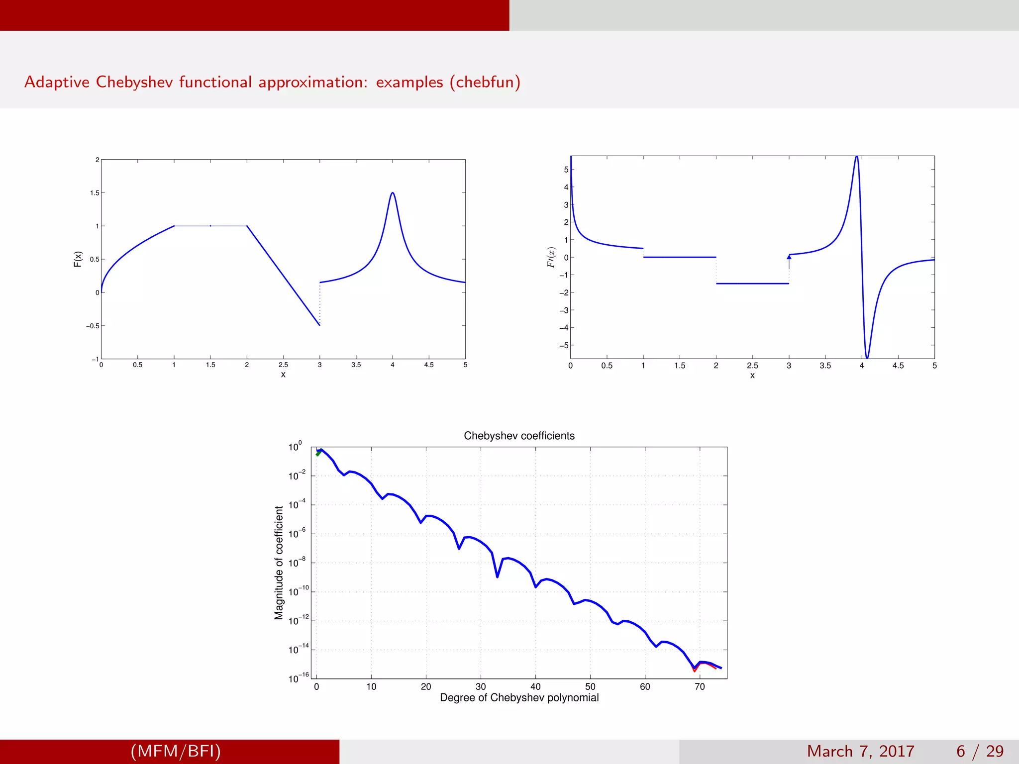
5. Adaptive Chebyshev functional approximation (chebfun.org)
Given Chebyshev interpolation nodes zk , k = 1, . . . , m on [−1, 1]
zk = −cos
2k − 1
2m
π
and Chebychev coefficients ai , i = 0, . . . , n computed on Chebychev nodes we can approximate
F(x) ≈
n
i=0
ai Ti (x) ; ai =
2
π
1
−1
F(x)Ti (x)
1 − x2
dx
”Approximation Theory and Approximation Practice”, by Lloyd N. Trefethen (chebfun.org)
”Chebyshev and Fourier Spectral Methods”, by John P. Boyd
Chebyshev interpolation nodes and degree of polynomials have to be adaptive during continuous Newton updates.
(i) When in doubt, use Chebyshev polynomials unless the solution is spatially periodic, in which case an ordinary Fourier
series is better.
(ii) Unless youre sure another set of basis functions is better, use Chebyshev polynomials.
(iii) Unless youre really, really sure that another set of basis functions is better, use Chebyshev polynomials
(MFM/BFI) March 7, 2017 5 / 29

6. Adaptive Chebyshev functional approximation: examples (chebfun)
0 0.5 1 1.5 2 2.5 3 3.5 4 4.5 5
−1
−0.5
0
0.5
1
1.5
2
x
F(x)
0 0.5 1 1.5 2 2.5 3 3.5 4 4.5 5
−5
−4
−3
−2
−1
0
1
2
3
4
5
x
F′(x)
0 10 20 30 40 50 60 70
10
−16
10
−14
10
−12
10
−10
10
−8
10
−6
10
−4
10
−2
10
0
Chebyshev coefficients
Degree of Chebyshev polynomial
Magnitudeofcoefficient
(MFM/BFI) March 7, 2017 6 / 29

7. shock-exposure and shock-price elasticity
first kind
Multiplicative functional Mt :
1) consumption Ct for consumption shock-exposure
2) stochastic discount factor St for consumption shock-price elasticity
d log Mt = β(Xt )dt + α(Xt )dBt
(x, t) = σ(x)
∂
∂x
log E[Mt |X0 = x] + α(x)
Define
φ(x, t) = E
Mt
M0
|X0 = x
Then solve PDE
∂φ(x, t)
∂t
=
1
2
σ
2
(x)
∂2
∂x2
φ(x, t) + (µ(x) + σ(x)α(x))
∂
∂x
φ(x, t) + β(x) +
1
2
|α(x)
2
| φ(x, t)
s.t. initial boundary condition φ(x, 0) = 1
(MFM/BFI) March 7, 2017 7 / 29

8. shock-exposure and shock-price elasticity
second kind
Multiplicative functional Mt :
1) consumption Ct for consumption shock-exposure
2) stochastic discount factor St for consumption shock-price elasticity
d log Mt = β(Xt )dt + α(Xt )dBt
The elasticity of second kind is
2(Xt ) =
E(Dt Mt )|F0
EMt |F0
Use specification for Mt to get
2(Xt ) =
E( Mt η(Xt )α(Xt ))|F0
EMt |F0
Then solve PDE twice
∂φ(x, t)
∂t
=
1
2
σ
2
(x)
∂2
∂x2
φ(x, t) + (µ(x) + σ(x)α(x))
∂
∂x
φ(x, t) + β(x) +
1
2
|α(x)
2
| φ(x, t)
s.t. initial boundary condition φ(x, 0) = 1 to get a solution φ1(x, t) and initial boundary condition φ(x, 0) = α(x) to get a
solution φ2(x, t) Then, second type elasticity is
2(x, t) =
φ2(x, t)
φ1(x, t)
(MFM/BFI) March 7, 2017 8 / 29

9. ”Intermediary Asset Pricing”: Zhiguo He and Arvind Krishnamurthy, AER, 2013
Find
Pt
Dt
= F(y), ∀y ∈ 0, 1+l
ρ
, by solving
F (y) θs (y)G (y)
2 (θb (y)σ)2
2
G (y)
θs (y)F (y)
1 + l + ρy(γ − 1)
1 + l − ρy + ργG (y) θb (y)
= ρ + g(γ − 1) −
1
F (y)
+
γ (1 − γ) σ2
2
1 +
ρG (y) θb (y)
1 + l − ρy
y − G (y) θb (y)
θs (y)F (y)
1 + l − ρy − ρG (y) θb (y)
1 + l − ρy + ργG (y) θb (y)
−
(1 + l − ρy) (G (y) − 1)
θs (y)F (y)
+ γρG (y)
θs (y) + l + θb (y)(g(γ − 1) + ρ) − ρy
1 + l − ρy + ργG (y) θb (y)
.
where
G (y) =
1
1 − θs (y)F (y)
,
and
if y ∈ (0, yc
) if y ∈ yc
, 1+l
ρ
θs (y) =
(1−λ)y
F(y)−λy
m
1+m
θb (y) = λy
F(y)−y
F(y)−λy
y − m
1+m
F (y)
.
The endogenous threshold yc
is determined by yc
= m
1−λ+m
F (yc
). Boundary conditions on y = 0 and y = 1+l
r
.
F (0) =
1 + F (0) l
ρ + g(γ − 1) +
γ(1−γ)σ2
2
− lγρ
1+l
; F
1 + l
ρ
=
1 + l
ρ
; F
1 + l
ρ
= 1.
(MFM/BFI) March 7, 2017 9 / 29

10. He-Krishnamurthy, BVP solution
dXt = µy (Xt )dt + σy (Xt )dBt , Xt =
wt
Pt
; σy (Xt ) = −
θb
1 − θs F (y)
σ; Xt =
F(y) − y
F(y)
d log Ct = β(Xt )dt + α(Xt )dBt ; d log St = −γ log Ct
β(x) = µ(x)ξ(x) +
1
2
σ(x)
2 ∂ξ
∂x
+ gd −
σ2
d
2
; α(x) = σ(x)ξ(x) + σd ; ξ(x) = −ρ
p (x)(1 − x) − p(x)
1 + l − ρ(1 − x)p(x)
0 0.2 0.4 0.6 0.8 1
−0.05
0
0.05
0.1
0.15
0.2
X
µ(X)
0 0.2 0.4 0.6 0.8 1
0
0.05
0.1
0.15
0.2
X
σ(X)
(MFM/BFI) March 7, 2017 10 / 29

11. example, He-Krishnamurthy
stationary density distribution, percentiles
*
X
0 0.1 0.2 0.3 0.4 0.5 0.6
stationarydensity
0
2
4
6
8
10
12
density
1%
5%
25%
35.3%
50%
75%
90%
99%
(MFM/BFI) March 7, 2017 11 / 29

12. He-Krushnamurthy: shock exposure, specialist C
(a) type 1 elasticity (b) type 2 elasticity
(MFM/BFI) March 7, 2017 12 / 29

13. He-Krushnamurthy: price exposure, specialist C
(a) type 1 elasticity (b) type 2 elasticity
(MFM/BFI) March 7, 2017 13 / 29

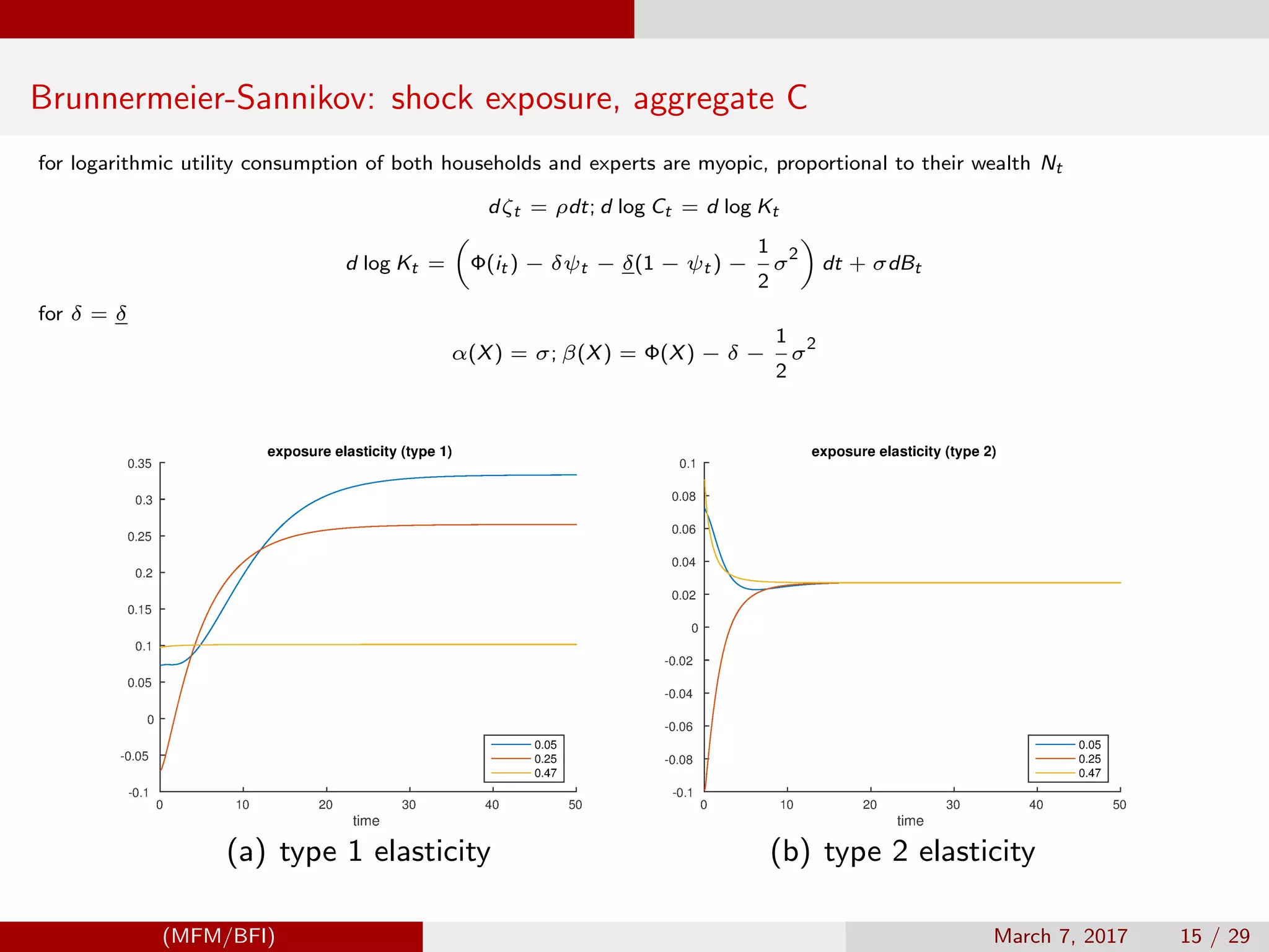
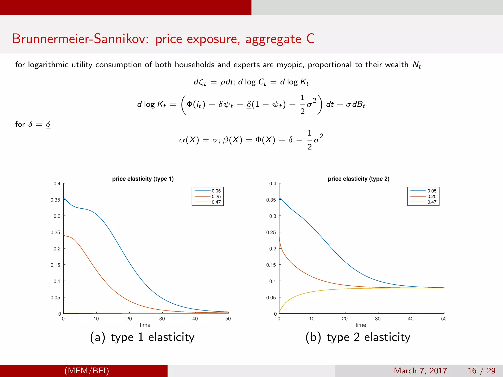
14. Brunnermeier-Sannikov example
dXt
Xt
= µ(Xt )dt + σ(Xt )dBt − dζt , Xt =
Nt
qt Kt
;
X(t) : expert share of wealth
Consumption is aggregate output net of aggregate investment
C
a
t = [aψ(Xt ) + a(1 − ψ(Xt ))]Kt
d log Ct = β(Xt )dt + α(Xt )dBt ;
where
α(X) = σ; β(X) = Φ(X) − δ − σ
2
/2
For log-utility
St /S0 = e
−ρt
C0/Ct
(MFM/BFI) March 7, 2017 14 / 29

15. Brunnermeier-Sannikov: shock exposure, aggregate C
for logarithmic utility consumption of both households and experts are myopic, proportional to their wealth Nt
dζt = ρdt; d log Ct = d log Kt
d log Kt = Φ(it ) − δψt − δ(1 − ψt ) −
1
2
σ
2
dt + σdBt
for δ = δ
α(X) = σ; β(X) = Φ(X) − δ −
1
2
σ
2
(a) type 1 elasticity (b) type 2 elasticity
(MFM/BFI) March 7, 2017 15 / 29

16. Brunnermeier-Sannikov: price exposure, aggregate C
for logarithmic utility consumption of both households and experts are myopic, proportional to their wealth Nt
dζt = ρdt; d log Ct = d log Kt
d log Kt = Φ(it ) − δψt − δ(1 − ψt ) −
1
2
σ
2
dt + σdBt
for δ = δ
α(X) = σ; β(X) = Φ(X) − δ −
1
2
σ
2
(a) type 1 elasticity (b) type 2 elasticity
(MFM/BFI) March 7, 2017 16 / 29

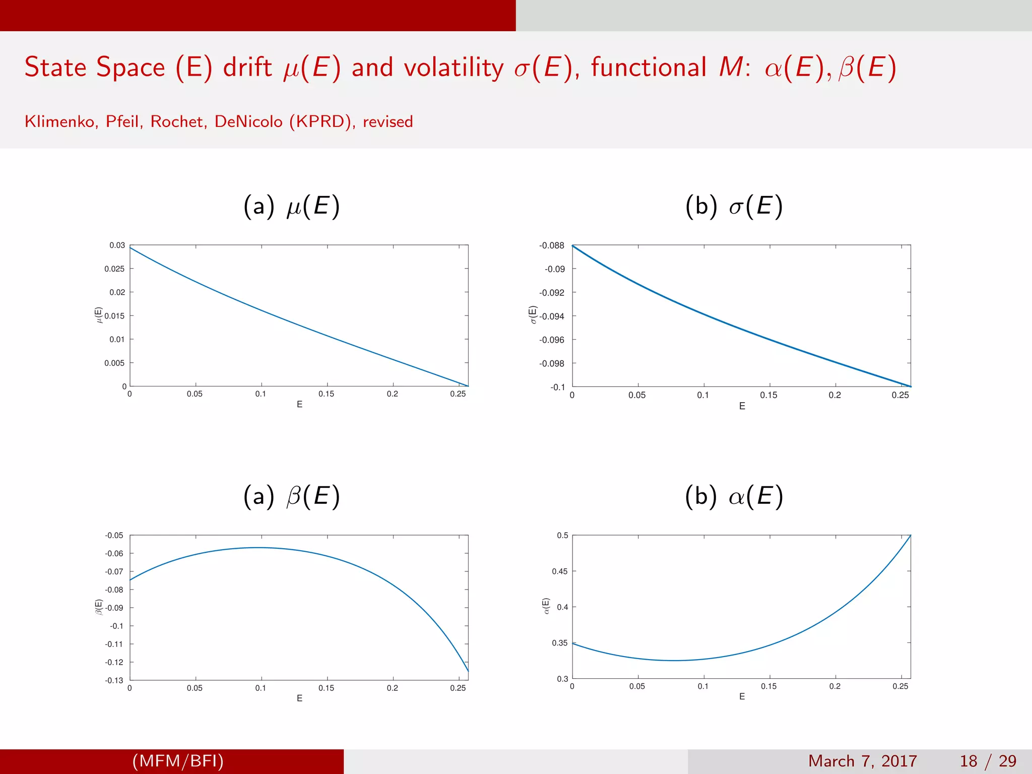
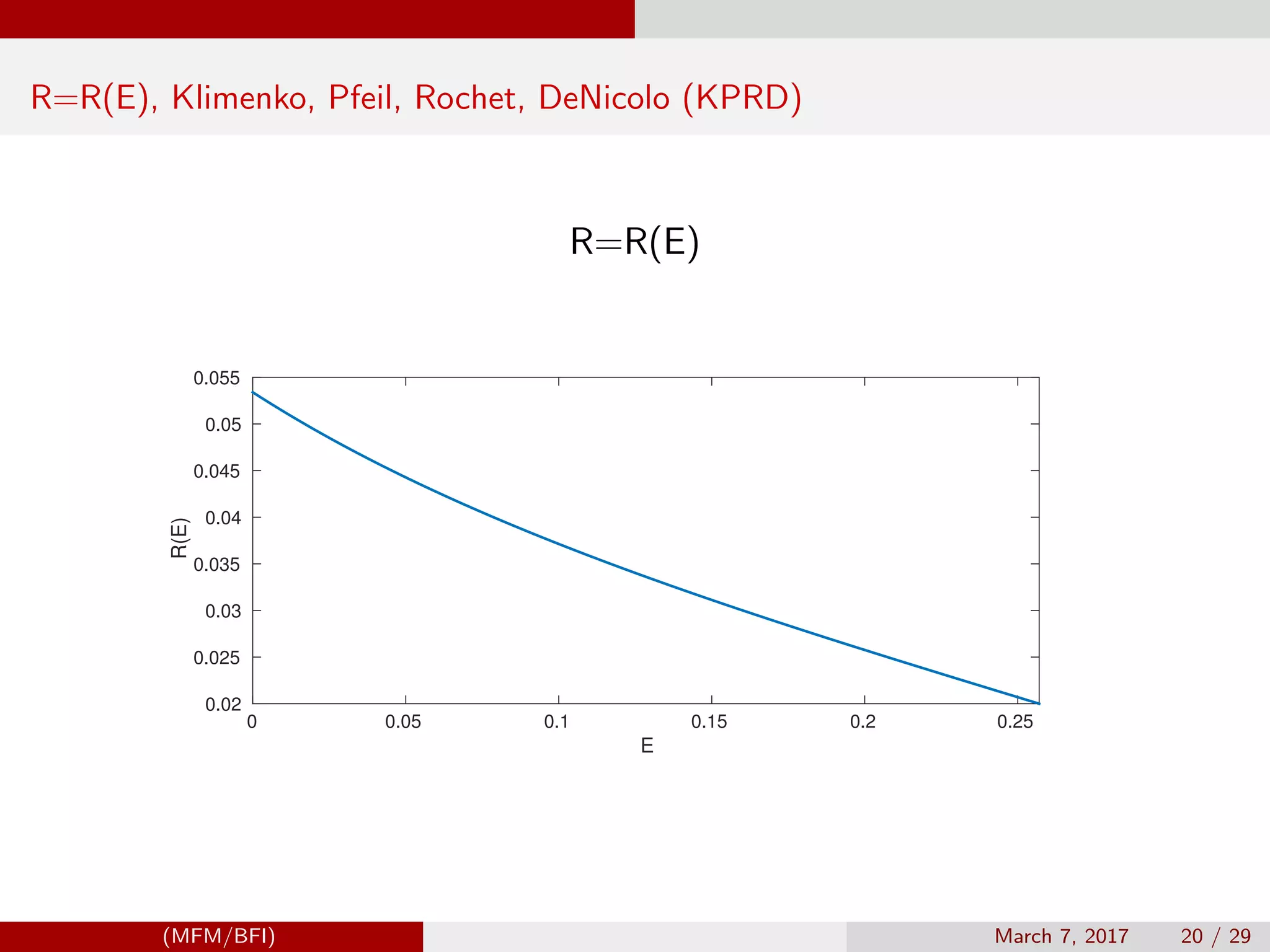
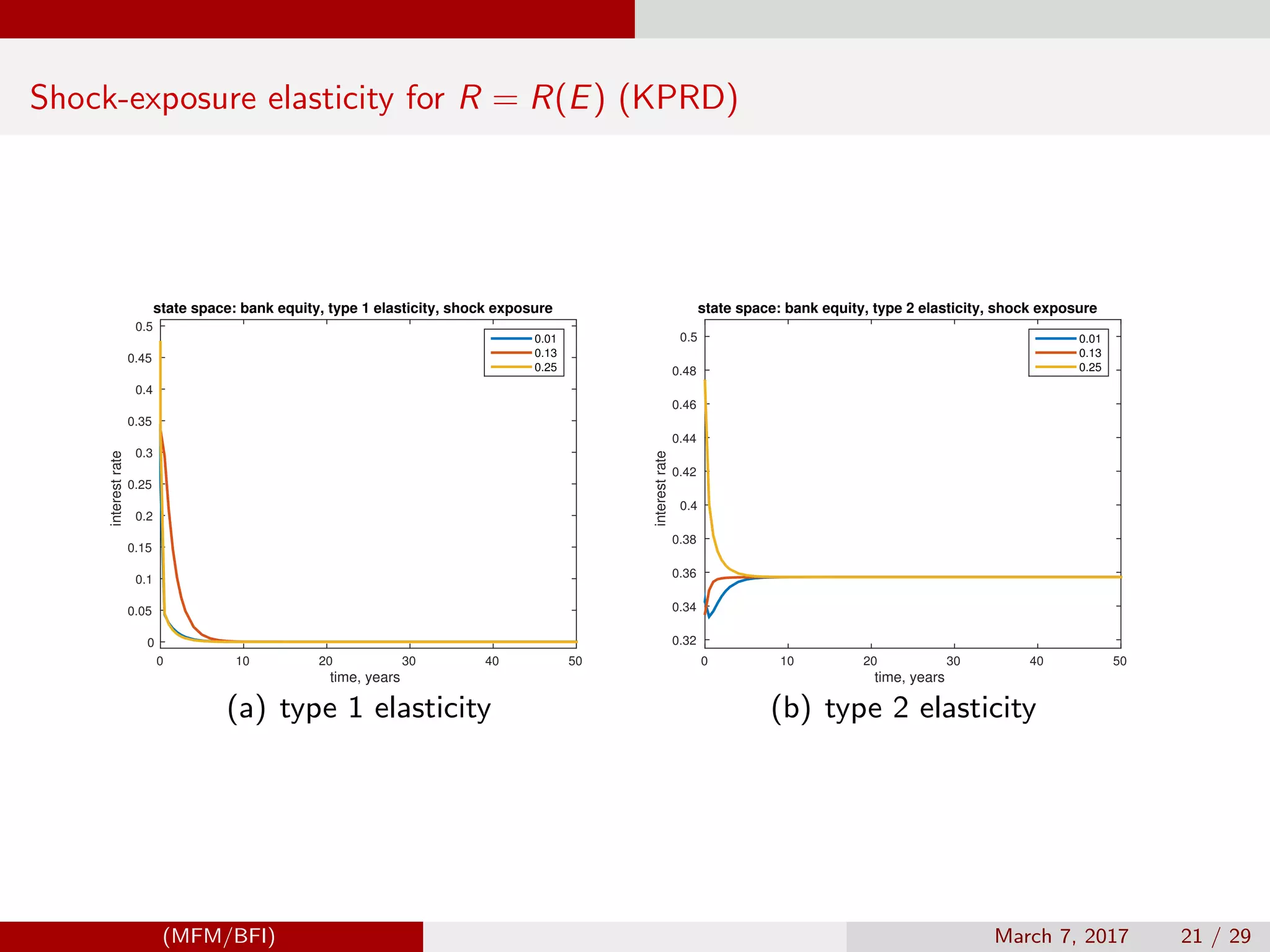
17. Model Settings, Klimenko, Pfeil, Rochet, DeNicolo (KPRD)
State - equity E
Multiplicative functional M = R(E)
dEt = µ(Et )dt + σ(Et )dBt , p + r ≤ Rt ≤ Rmax ,
where
µ(E) = Er + L(R(E))(R(E) − r − p); σ(E) = L(R(E))σ0.
Emax
0
R(s) − p − r
σ2
0L(R(s))
ds = ln(1 + γ); u(E) = exp
Emax
E
R(s) − p − r
σ2
0L(R(s))
ds
with
L(R) =
R − R
R − p
β
where u(E) is market-to-book value
d log R =
R(E)
R(E)
dE = ψ(E)dE → d log Rt = β(Et )dt + α(Et )dBt
where β(E) = µ(E)ψ(E) + 1
2
σ(E)2 ∂ψ(E)
∂E
, α(E) = σ(E)ψ(E); s.t. Neumann b.c.:
∂φt (E)
∂x
Emin,max
= 0
R (E) = −
1
σ2
0
2(ρ − r)σ2
0 + [R(E) − p − r]2
+ 2rE[R(E) − p − r]L(R(E))−1
L(R(E)) − L (R(E))[R(E) − p − r]
, R(Emax ) = p + r
(MFM/BFI) March 7, 2017 17 / 29

18. State Space (E) drift µ(E) and volatility σ(E), functional M: α(E), β(E)
Klimenko, Pfeil, Rochet, DeNicolo (KPRD), revised
(a) µ(E)
E
0 0.05 0.1 0.15 0.2 0.25
µ(E)
0
0.005
0.01
0.015
0.02
0.025
0.03
(b) σ(E)
E
0 0.05 0.1 0.15 0.2 0.25
σ(E)
-0.1
-0.098
-0.096
-0.094
-0.092
-0.09
-0.088
(a) β(E)
E
0 0.05 0.1 0.15 0.2 0.25
β(E)
-0.13
-0.12
-0.11
-0.1
-0.09
-0.08
-0.07
-0.06
-0.05
(b) α(E)
E
0 0.05 0.1 0.15 0.2 0.25
α(E)
0.3
0.35
0.4
0.45
0.5
(MFM/BFI) March 7, 2017 18 / 29

19. stationary density in E and R, Klimenko, Pfeil, Rochet, DeNicolo (KPRD)
in E space
E
0 0.05 0.1 0.15 0.2 0.25 0.3
0
1
2
3
4
5
stationary density
in R space (identical to a graph in KPRD paper)
R
0.02 0.025 0.03 0.035 0.04 0.045 0.05 0.055
g(R)
0
5
10
15
20
25
30
35
40
45
(MFM/BFI) March 7, 2017 19 / 29

20. R=R(E), Klimenko, Pfeil, Rochet, DeNicolo (KPRD)
R=R(E)
E
0 0.05 0.1 0.15 0.2 0.25
R(E)
0.02
0.025
0.03
0.035
0.04
0.045
0.05
0.055
(MFM/BFI) March 7, 2017 20 / 29

21. Shock-exposure elasticity for R = R(E) (KPRD)
time, years
0 10 20 30 40 50
interestrate
0
0.05
0.1
0.15
0.2
0.25
0.3
0.35
0.4
0.45
0.5
state space: bank equity, type 1 elasticity, shock exposure
0.01
0.13
0.25
(a) type 1 elasticity
time, years
0 10 20 30 40 50interestrate
0.32
0.34
0.36
0.38
0.4
0.42
0.44
0.46
0.48
0.5
state space: bank equity, type 2 elasticity, shock exposure
0.01
0.13
0.25
(b) type 2 elasticity
(MFM/BFI) March 7, 2017 21 / 29

22. SDF and price elasticity, Klimenko, Pfeil, Rochet, DeNicolo (KPRD)
State - equity E
Multiplicative functional for SDF M = u(E)
u(E) = exp
Emax
E
R(s) − p − r
σ2
0L(R(s))
ds
with
L(R) =
R − R
R − p
β
where u(E) is market-to-book value
E
0 0.05 0.1 0.15 0.2 0.25 0.3
market-to-book
1
1.1
1.2
1.3
1.4
1.5
E
0 0.05 0.1 0.15 0.2 0.25 0.3
R(E)
0.02
0.03
0.04
0.05
0.06
(MFM/BFI) March 7, 2017 22 / 29

23. Price elasticity for R = R(E) (KPRD)
time, years
0 10 20 30 40 50
interestrate
-0.3
-0.25
-0.2
-0.15
-0.1
-0.05
0
state space: bank equity, type 1 elasticity, price exposure
0.01
0.13
0.25
(a) type 1 elasticity
time, years
0 10 20 30 40 50
interestrate
-0.3
-0.25
-0.2
-0.15
-0.1
-0.05
0
state space: bank equity, type 2 elasticity, price exposure
0.01
0.13
0.25
(b) type 2 elasticity
(MFM/BFI) March 7, 2017 23 / 29

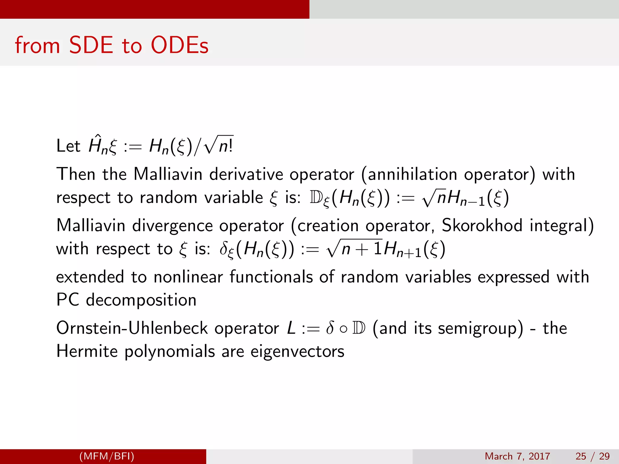
24. Malliavin Derivative
and Generalized Polynomial Chaos Expansion (gPC)
Fast technique for high-precision numerical analysis of stochastic non-linear systems
Malliavin calculus to integrate and differentiate processes that are expressed in generalized Polynomial Chaos (gPC)
Generating function
exp sx −
s2
2
=
∞
n=0
sn
n!
Hn(x); Hn(x) are orthogonal Hermite polynomials
Let Bt be Brownian motion, Mt = exp sBt − s2t
2
Then (Ito)
dMt = s
∞
n=0
sn
n!
xn(t)dBt , xn(t) = t
n/2
Hn(Bt /
√
t)
dxn(t) = nxn−1dBt ; xn(t) = n!
t
0
dB(tn−1)
tn−1
0
dB(tn−2) . . .
t2
0
dB(t1)
u(t, Bt ) ≈
p
i=0
ui (t)Hi (Bt ), Cameron and Martin for Gaussian random variables, Xiu-Karniadakis for generalized
u0(x, t) = E[u(x, t, ξ)H0] = E[u(x, t, ξ)]
(MFM/BFI) March 7, 2017 24 / 29

25. from SDE to ODEs
Let ˆHnξ := Hn(ξ)/
√
n!
Then the Malliavin derivative operator (annihilation operator) with
respect to random variable ξ is: Dξ(Hn(ξ)) :=
√
nHn−1(ξ)
Malliavin divergence operator (creation operator, Skorokhod integral)
with respect to ξ is: δξ(Hn(ξ)) :=
√
n + 1Hn+1(ξ)
extended to nonlinear functionals of random variables expressed with
PC decomposition
Ornstein-Uhlenbeck operator L := δ ◦ D (and its semigroup) - the
Hermite polynomials are eigenvectors
(MFM/BFI) March 7, 2017 25 / 29

26. from SDE to ODEs (cont)
Loan rate Rt = R(Et ):
dRt = µ(Rt )dt + σ(Rt )dBt , p ≤ Rt ≤ Rmax ,
Rt = r0 +
t
0
µ(Rτ )dτ +
t
0
σ(Rτ )dBτ
Rt ≈
p
i=0
ri (t)Hi (ξ); B(t, ξ) ≈
n
i=1
bi (t)Hi (ξ), ξ ∼ N(0, 1), {Hi } − Hermite polynomials : KLE
Integration by parts: E F t
0 Rτ dBτ = E t
0 DξFRτ dτ
˙ri (t) ≈ µ(Rt ) i +
n
j=1
jbj (t) σ(Rt ) j−1, i = 0, . . . , p
Non-linear IRF: Ft = D0Rt from Borovicka-Hansen-Scheinkman
(MFM/BFI) March 7, 2017 26 / 29

27. Stochastic Galerkin and Polynomial Chaos Expansion
for Stochastic PDE
Spectral expansion in stochastic variable(s): ξ ∈ Ω:
u(x, t, ξ) =
∞
i=0
ui (x, t)ψi (ξ)
where ψi (ξ) are orthogonal polynomials (Hermite, Legendre, Chebyshev)
standard approximations (spectral or finite elements) in space and polynomial (also spectral or pseudo-spectral) approximation in
the probability domain
Babuska, Ivo, Fabio Nobile, and Raul Tempone. ”A stochastic collocation method for elliptic partial differential equations with
random input data.” SIAM Journal on Numerical Analysis 45.3 (2007): 1005-1034.
u(x, t, ξ) ≈
p
i=0
ui (x, t)ψi (ξ)
substitute into PDE and do a Galerkin projection by multiplying with ψk (ξ)
∂u
∂t
= a(ξ)
∂2
u
∂x2
;
p
i=0
∂ui (x, t)
∂t
ψi ψk +
p
i=0
∂2
ui
∂x2
pσ
j=0
aj ψj ψi ψk , k = 0, . . . , p
(MFM/BFI) March 7, 2017 27 / 29

28. Monte-Carlo/gPC comparison (sglib)
gPC expansion for ln N(µ, σ2
) with µ = 0.03, σ = 0.85, comparison with exact value and MC (1,000 and 100,000 samples)
(MFM/BFI) March 7, 2017 28 / 29

29. Extension to many dimensions:
Adaptive sparse (Smolyak) grids (Bocola, 2015), tensor approximation
−1 −0.5 0 0.5 1
−1
−0.5
0
0.5
1
−1 −0.5 0 0.5 1
−1
−0.5
0
0.5
1
−1 −0.5 0 0.5 1
−1
−0.5
0
0.5
1
−1 −0.5 0 0.5 1
−1
−0.5
0
0.5
1
−1
0
1
−1
0
1
−1
0
1
−1
0
1
−1
0
1
−1
0
1
−1
0
1
−1
0
1
−1
0
1
−1
0
1
−1
0
1
−1
0
1
Tensor-train decomposition (TT Toolbox)
A(i1, . . . , id ) = G1(i1)G2(i2) . . . Gd (id ),
where Gk (ik ) is rk−1 × rk , r0 = rd = 1.
basic linear algebra operations in O(dnrα
)
rank reduction in O(dnr3
) operations
tensor can be recovered exactly by sampling
(MFM/BFI) March 7, 2017 29 / 29