fgh drt jkl

1. WORK SAMPLING AND
STRUCTURED ESTIMATING

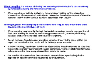
2. Work sampling is a method of finding the percentage occurrence of a certain activity
by statistical sampling and random observations.
• Work sampling, or activity analysis, is the process of making sufficient random
observations of an operator’s activities to determine the relative amount of time the
operator spends on the various activities associated with the job.
The major goal of work sampling is to determine how long, or how much of the work
day, is spent on specific types of work.
• Work sampling may identify the fact that certain operators spend a large portion of
their time waiting for work, or performing paperwork tasks, or even performing
activities that are not included in their job descriptions.
• One of the basic foundations of statistical sampling theory is the concept that the
larger the sample size, the results will be better or more accurate.
• In work sampling, a sufficient number of observations must be made to be sure that
the results accurately summarize the work performed. There are statistical formulas
to help determine how many observations should be made.
• The number of observations that an analyst must make of a particular job also
depends on how much time is devoted to a particular task.

3. CONDUCTING A STUDY
• It is recommended that a uniform procedure should be followed to perform a work
sampling study is to
1. Establish the Purpose
• First, the objective of the study should be established. Work sampling can be used to
determine an overall perspective on the work done.
2. Identify the Subjects
• Second, the people performing the task must be identified, i.e. general office work is being
studied with the objective of determining overall productivity.
3. Identify the Measure of Output
• The third step in making the study is the identification of the measure of the output
produced or the types of activities performed on the jobs being studied. This step is
especially important if the objective of the study is to measure productivity with the intent
of setting a standard.
4. Establish a Time Period
• Fourth, the time period during which the study will be conducted must be established.
Starting and stopping points for the study must be defined as well.
5. Define the Activities
• This step involves defining the activities that are performed by the people under study. For
example, the definition used in a machine utilization study, including only the categories of
working, idle, and idle-mechanical breakdown.

4. 6. Determine the Number of Observations Needed
• After the work elements are defined, the number of observations for the desired accuracy at the desired
confidence level must be determined. The sample size is dependent on the percentage of time believed to
be spent on the major work element.
• If a reasonable guess cannot be made, then a trial study of perhaps 20 to 40 observations should be made
to get an estimate of this portion. These initial observations should be included with the rest of the
observations taken during the rest of the work study.
7. Schedule the Observations
• Once the number of required observations has been determined, either from appropriate statistical
calculations or from tables, the actual observations must be scheduled. Typically, the analyst will assign an
equal number of observations each day during the course of the study.
• For example, if 800 observations are required and 20 work days are established as an appropriate
observation time, 40 observations should be recorded each day.
• A random number table can be used to establish the random times for each observation.
8. Inform the Personnel Involved
• Before the study is actually performed, the personnel involved should be informed about the objective of
the study and the methodology that will be employed. As in any productivity measurement study, this part
of the procedure is very important.
• Workers and their supervisors might think that they personally are being measured rather than the work
they are doing.
9. Record the Raw Data
• The next and perhaps the easiest part of any work sampling study is the actual recording of the raw data.
Although this recording can be performed by anyone, it is desirable that a trained analyst be employed.
• It is also very important that the observations be made at exactly the same location every time. Failure to
be reliable in this manner may bias the results.
10. Summarize the Data
• After the data have been collected, they must be summarized.

5. A few words about sampling
• Sampling is mainly based on probability. Probability has been defined as “the
degree to which an event is likely to occur”.
• A simple and often-mentioned example that illustrates the point is that of
tossing a coin.
• The law of probability says that we are likely to have 50 heads and 50 tails in
every 100 tosses of the coin. The greater the number of tosses, the more chance
we have of arriving at a ratio of 50 heads to 50 tails.
• The size of the sample is therefore important, and we can express our
confidence in whether or not the sample is representative by using a certain
confidence level.
Establishing confidence levels
• Let us go back to our previous example and toss five coins at a time, and then
record the number of times we have heads and the number of times we have
tails for each toss of these five coins. Let us then repeat this operation 100
times.
• If we considerably increase the number of tosses and in each case toss a large
number of coins at a time, we can obtain a smoother curve, such as that shown
in figure 89.

7. • To make things easier, it is more convenient to speak of a 95 per cent confidence level than of a
95.45 per cent confidence level.
• To achieve this we can change our calculations and obtain:
– 95 per cent confidence level or 95 per cent of the area under the curve = 1.96
– 99 per cent confidence level or 99 per cent of the area under the curve = 2.58
– 99.9 per cent confidence level or 99.9 per cent of the area under the curve = 3.3
• In this case we can say that if we take a large sample at random we can be confident that in 95

8. Determination of sample size
• As well as defining the confidence level for our observations we have to decide
on the margin of error that we can allow for these observations.
• Let us look at our example about the productive time and the idle time of the
machines in a factory. There are two methods of determining the sample size
that would be appropriate for this example:
• the statistical method and the nomogram method.
Statistical method. The formula used in this method is:

9. • Let us assume that some 100 observations were carried out as a preliminary study and at
random, and that these showed the machine to be idle in 25 per cent of the cases (p = 25)
and to be working 75 per cent of the time (q = 75).
• We thus have approximate values for p and q; in order now to determine the value of n,
we must find out the value of .
• Let us choose a confidence level of 95 per cent with a 10 per cent margin of error (that is,
we are confident that in 95 per cent of the cases our estimates will be ± 10 per cent of the
real value).

10. Nomogram method
An easier way to determine sample size is to read off the number of observations needed
directly from a nomogram such as the one reproduced in figure 91.

11. Making random observations
• To ensure that our observations are in fact made at random, we can use a
random table such as the one in table 12.
• Various types of random table exist, and these can be used in different
ways. In our case let us assume that we shall carry out our observations
during a day shift of eight hours, from 7 a.m. to 3 p.m. An eight-hour day
has 480 minutes. These may be divided into 48 ten-minute periods.
• We can start by choosing any number at random from our table, for
example by closing our eyes and placing a pencil point somewhere on the
table. Let us assume that in this case we pick, by simple chance, the
number 11 which is in the second block, fourth column, fourth row (table
12).
• We now choose any number between 1 and 10. Assume that we choose
the number 2; we now go down the column picking out every second
reading and noting it down, as shown below (if we had chosen the number
3, we should pick out every third figure, and so on).
• 11 38 45 87 68 20 11 26 49 05

13. • Looking at these numbers, we find that we have to discard 87, 68 and 49 because they are
too high (since we have only 48 ten-minute periods, any number above 48 has to be
discarded).
• Similarly, the second 11 will also have to be discarded since it is a number that has already
been picked out. We therefore have to continue with our readings to replace the four
numbers we have discarded. Using the same method, that is choosing every second
number after the last one (05), we now have14 15 47 22
• These four numbers are within the desired range and have not appeared before. Our final
selection may now be arranged numerically and the times of observation throughout the
eight-hour day worked out. Thus our smallest number (05) represents the fifth ten-minute
period after the work began at 7 a.m. Thus our first observation will be at 7.50 a.m., and so
on (table 13).

14. Example: Conducting the study
• Determining the scope of the study. Before making our actual observations, it is important that
we decide on the objective of our work sampling.
• The simplest objective is that of determining whether a given machine is idle or working.
• In such a case, our observations aim at detecting one of two possibilities only:
• We can, however, extend this simple model to try to find out the cause of the stoppage of the
machine:

15. Making the observations
• So far we have taken the first five logical steps in conducting a work
sampling study.
– selecting the job to be studied and determining the objectives of the
study;
– making a preliminary observation to determine the approximate values
of p and q;
– in terms of a chosen confidence level and accuracy range, determining
n (the number of observations needed) determining the frequency of
observations, using random tables;
– designing record sheets to meet the objectives of the study.
– There is one more step to take: that of making and recording the
observations and analyzing the results.

17. Group sampling techniques
• As the name suggests, these are designed for the measurement of work
carried out by groups of workers.
• The techniques are sometimes referred to by the term “high-frequency
sampling” since, when used for the measurement of short-cycle work, they
use fixed short-time intervals with the observer in constant attendance.
• They are very close to time study but have the advantage that the observer
can cover the work of the group. Group sampling techniques may make use
of rating.
• Consider a very simple example of three workers each producing the same
parts by a process that involves only hand tools. The sampling is carried out
at 0.5 minute intervals and involves the categories of “working” and “not
working” only.
• The sampling observations have been rated and this is an example of both
rated activity sampling and group sampling.
• The sampling sheet would look as shown in table 14.