2. I. Aljarah et al.
swarm-based algorithms, which are the two main families of
meta-heuristic algorithms, are among the most investigated
methods by researchers in training MLP networks. These
types of algorithms are population based, in which a num-
ber possible random solutions are generated, evolved, and
updated until a satisfactory solution is found or a maximum
number of iterations is reached. These algorithms incorpo-
rate randomness as the main mechanism to move from a local
search to a global search, and therefore, they are more suit-
able for global optimization (Yang 2014).
Evolutionary algorithms were deployed in the supervised
learning of MLP networks in three different main schemes:
automatic design of the network structure, optimizing the
connection weights and biases of the network, and evolv-
ing the learning rules (Jianbo et al. 2008). It is important to
mention here that simultaneous optimization of the structure
and weights of the MLP network can drastically increase the
number of parameters, so it can be considered a large-scale
optimization problem (Karaboga et al 2007). In this work,
we focus only on optimizing the connection weights and the
biases in the MLP network.
Genetic algorithm (GA) is a classical example of evo-
lutionary algorithms and considered as one of the most
investigated meta-heuristics in training neural networks.
GA is inspired by the Darwinian theories about evolution
and nature selection, and it was first proposed by Holland
(1992), Goldberg (1989), and Sastry et al (2014). In Seif-
fert (2001), the author applied GA to train the connection
weights in MLP network and argued that GA can outperform
the back-propagation algorithm when the targeted problems
are more complex. A similar approach was conducted in
Gupta and Randall (1999) where GA was compared to back-
propagation for the chaotic time-series problems, and it was
shown that GA is superior in terms of effectiveness, ease
of use, and efficiency. Other works on applying GA to train
MLP networks can be found in Whitley et al. (1990), Ding
et al. (2011), Sexton et al. (1998), and Randall (2000). Differ-
ential evolution (DE) (Storn and Price 1997; Price et al 2006;
Das and Suganthan 2011) and evolution strategy (ES) (Beyer
and Schwefel 2002) are other examples of evolutionary algo-
rithms. DE and ES were applied in training MLP networks
and compared to other techniques in different studies (Wdaa
2008; Ilonen et al. 2003; Slowik and Bialko 2008; Wienholt
1993). Another distinguished type of meta-heuristics that is
getting more interest is the swarm-based stochastic search
algorithms, which are inspired by the movements of birds,
insects, and other creatures in nature. Most of these algo-
rithms incorporate updating the generated random solutions
by some mathematical models rather than the reproduction
operators like those in GA. The most popular examples of
swarm-based algorithms are the particle swarm optimization
(PSO) (Zhang et al. 2015; Kennedy 2010), ant colony opti-
mization (ACO) (Chandra 2012; Dorigo et al. 2006), and the
artificial bee colony (ABC) (Karaboga et al. 2014; Karaboga
2005). Some interesting applications of these algorithms and
their variations in the problem of training MLP networks are
reported in Jianbo et al. (2008), Mendes et al (2002), Meiss-
ner et al. (2006), Blum and Socha (2005), Socha and Blum
(2007), and Karaboga et al (2007).
Although a wide range of evolutionary and swarm-based
algorithms are deployed and investigated in the literature
for training MLP, the problem of local minima is still open.
According to the no-free-lunch theorem (NFL), there is no
superior optimization algorithm in all optimization problems
(Wolpert and Macready 1997; Ho and Pepyne 2002). Moti-
vated by these reasons, in this work, a new MLP training
method based on the recent whale optimization algorithm
(WOA) is proposed for training a single hidden layer neural
network. WOA, a novel meta-heuristic algorithm, was first
introduced and developed in Mirjalili and Lewis (2016).
WOA is inspired by the bubble-net hunting strategy of hump-
back whales. Unlike previous works in the literature where
the proposed training algorithms are tested on roughly five
datasets, the developed WOA-based approach in this work
is evaluated and tested based on 20 popular classification
datasets. Also, the results are compared to those obtained for
basic trainers from the literature including: four evolutionary
algorithms (GA, DE, ES and the population-based incre-
mental learning algorithm (PBIL) (Baluja 1994; Meng et al.
2014), two swarm intelligent algorithms (PSO and ACO),
and the most popular gradient-based back-propagation algo-
rithm.
This paper is organized as follows: A brief introduction to
MLP is given in Sect. 2. Section 3 presents the WOA. The
details of the proposed WOA trainer are described and dis-
cussed in Sect. 4. The experiments and results are discussed
in Sect. 5. Finally, the findings of this research are concluded
in Sect. 6.
2 Multilayer perceptron neural network
Feedforward neural networks (FFNNs) are a special form
of supervised neural networks. FFNNs consist of a set of
processing elements called ‘neurons.’ The neurons are dis-
tributed over a number of stacked layers where each layer is
fully connected with next one. The first layer is called the
input layer, and this layer maps the input variables to the
network. The last layer is called the output layer. All layers
between the input layer and the output layer are called hid-
den layers (Basheer and Hajmeer 2000; Panchal and Ganatra
2011).
Multilayerperceptron(MLP)isthemostpopularandcom-
mon type of FFNN. In MLP, neurons are interconnected in
a one-way and one-directional fashion. Connections are rep-
resented by weights which are real numbers that fall in the
123
3. Optimizing connection weights in neural networks using the whale optimization algorithm
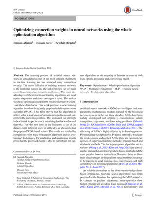
Fig. 1 Multilayer perceptron neural network
interval [−1, 1]. Figure 1 shows a general example of MLP
with only one hidden layer. The output of each node in the
network is calculated in two steps. First, the weighted sum-
mation of the input is calculated using Eq. 1 where Ii is the
input variable i, while wi j is the connection weight between
Ii and the hidden neuron j.
Second, an activation function is used to trigger the output
of neurons based on the value of the summation function.
Different types of activation functions could be used in MLP.
Using the sigmoid function, which is the most applied in the
literature, the output of the node j in the hidden layer can be
calculated as shown in Eq. 2 .
Sj =
n
i=1
wi j Ii + βj (1)
f j (x) =
1
1 + e−Sj
(2)
After calculating the output of each neuron in the hidden
layer, the final output of the network is calculated as given in
Eq. 3.
ˆyk =
m
i=1
Wkj fi + βk (3)
3 The whale optimization algorithm
Whale optimization algorithm (WOA) is a recently proposed
stochasticoptimizationalgorithm(Mirjalili andLewis 2016).
It utilizes a population of search agents to determine the
globaloptimumforoptimizationproblems.Similarlytoother
population-based algorithms, the search process starts with
creating a set of random solutions (candidate solutions) for a
given problem. It then improves this set until the satisfaction
Fig. 2 Bubble-net hunting behavior
of an end criterion. The main difference between WOA and
other algorithms is the rules that improve the candidate solu-
tions in each step of optimization. In fact, WOA mimics the
hunting behavior of hump back whales in finding and attack-
ing preys called bubble-net feeding behavior. The bubble-net
hunting model is shown in Fig. 2.
It may be observed in this figure that a humpback whale
creates a trap with moving in a spiral path around preys
and creating bubbles along the way. This intelligent foraging
method is the main inspiration of the WOA. Another simu-
lated behavior of humpback whales in WOA is the encircling
mechanism. Humpback whales circle around preys to start
hunting them using the bubble-net mechanism. The main
mathematical equation proposed in this algorithm is as fol-
lows:
X(t + 1) =
X∗(t) − AD p < 0.5
D eblcos(2πt) + X∗(t) p ≥ 0.5
(4)
where p is a random number in [0, 1], D = |X∗(t) − X(t)|
and indicates the distance of the ith whale the prey (best
solution obtained so far), b is a constant for defining the
shape of the logarithmic spiral, and l is a random number in
[−1, 1], t shows the current iteration, D = |CX∗(t) − X(t)|,
A = 2ar − a, C = 2r, a linearly decreases from 2 to 0 over
the course of iterations (in both exploration and exploitation
phases), and r is a random vector in [0, 1].
The first component of this equation simulates the encir-
cling mechanism, whereas the second mimics the bubble-net
technique. The variable p switches between these two com-
ponents with an equal probability. The possible positions of
a search agent using these two equations are illustrated in
Fig. 3.
The exploration and exploitation are two main phases of
optimization using population-based algorithms. They are
both guaranteed in WOA by adaptively tuning the parameters
a and c in the main equation.
123
4. I. Aljarah et al.
(X,Y)
(X*,Y*)
(X*,Y)
(X,Y*)
(X,Y*-AY)
(X*-AX,Y)
(X*,Y*-AY)(X*-AX,Y*-AY)
(X*-AX,Y*)
A=1
A=0.8
A=0.5
A=0.4
A=0.2
Fig. 3 Mathematical models for prey encircling and bubble-nethunting
The WOA starts optimizing a given problem by creating a
set of random solutions. In each step of optimization, search
agents update their positions based on a randomly selected
search agent or the best search agent obtained so far. To guar-
antee exploration and convergence, the best solution is the
pivot point to update the position of other search agents when
|X| > 1. In other situations (when |X| < 1), the best solu-
tion obtained so far plays the role of the pivot point. The
pseudocodes of the WOA are shown in Algorithm 1.
Algorithm 1 Pseudocodes of WOA
Initialize the whales population Xi (i = 1, 2, 3, ..., n)
Initialize a, A, and C
Calculate the fitness of each search agent
X∗ = the best search agent
procedure WOA(Population, a, A, C, Max Iter, .. )
t = 1
while t ≤ Max Iter do
for each search agent do
if |A| ≤ 1 then
Update the position of the current search
agent by the equation 2.6
else if |A| ≥ 1 then
Select a random search agent Xr and
Update the position of the current agent
by the equation 2.8
end if
end for
Update a, A, and C
Update X∗ if there is a better solution
t = t + 1
end while
return X∗
end procedure
It was proven by the inventors of WOA that this algorithm
is able to solve optimization problems of different kinds. It
was argued in the main paper that this is due to the flexibility,
gradient-free mechanism, and high local optima avoidance
of this algorithm. These motivated our attempts to employ
WOA as a trainer for FFNNs due to the difficulties of learn-
ing process. Theoretically speaking, WOA should be able to
train any ANN subject proper objective function and problem
formulation. In addition, providing the WOA with enough
number of search agents and iterations is another factor for
the success of this algorithm. The following section shows
how to train MLPs using WOA in details.
4 WOA for training MLP
In this section, we describe the proposed approach based on
the WOA for training the MLP network which will be named
as WOA-MLP. WOA is applied to train an MLP network with
a single hidden layer. Two important aspects are taken into
consideration when the approach is designed: the represen-
tation of the search agents in the WOA and the selection of
the fitness function.
In WOA-MLP, each search agent is encoded as a one-
dimensional vector to represent a candidate neural network.
Vectors include three parts: a set of weights connecting the
input layer with the hidden layer, a set of weights connecting
the hidden layer with the output layer, and a set of biases. The
length of each vectors equals the total number of weights and
biases in the network, and it can be calculated using Eq. 5
where is n is the number of input variables and m is the
number of neurons in the hidden layer.
Individual length = (n × m) + (2 × m) + 1 (5)
To measure the fitness value of the generated WOA agents,
we utilize the mean square error (MSE) fitness function
which is based on calculating the difference between the
actual and predicted values by the generated agents (MLPs)
for all the training samples. MSE is shown in Eq. 6 where y
is the actual value, ˆy is the predicted value, and n is number
of instances in the training dataset.
MSE =
1
n
n
i=1
(y − ˆy)2
(6)
123
5. Optimizing connection weights in neural networks using the whale optimization algorithm
Fig. 4 Assigning a WOA search agent vector to an MLP
The workflow of the WOA-based approach applied in this
work for training the MLP network can be described in the
following steps:
1. Initialization: A predefined number of search agents are
randomly generated. Each search agent represents a pos-
sible MLP network.
2. Fitness evaluation: The quality of the generated MLP
networks is evaluated using a fitness function. To per-
form this step, the set of weights and biases that form
the generated search agents vectors are first assigned to
MLP networks, and then each network is evaluated. In
this work, the MSE is selected, which is commonly cho-
sen as a fitness function in evolutionary neural networks.
The goal of the training algorithm is to find the MLP net-
work with the minimum MSE value based on the training
samples in the dataset.
3. Update the position of the search agents.
4. Steps 2 to 3 are repeated until the maximum number
of iterations is reached. Finally, the MLP network with
the minimum MSE value is tested on unseen part of the
dataset (test/validation samples).
The general steps of the WOA-MLPapproach are depicted
in Fig. 5.
5 Results and discussions
In this section, the proposed WOA approach for training
MLP networks is evaluated using twenty standard classifi-
Fig. 5 General steps of the WOA-MLP approach
cation datasets, which are selected from the University of
California at Irvine (UCI) Machine Learning Repository 1
and DELVE repository .2 Table 1 presents these datasets in
terms of the number of classes, features, training samples,
and test samples. As can be noticed, the selected datasets
have different numbers of features and instances to test the
training algorithms in different conditions, which makes the
problem more challenging.
5.1 Experimental setup
For all experiments, we used MATLAB R2010b to imple-
ment the proposed WOA trainer and other algorithms. All
datasets are divided into 66% for training and 34% for testing
using stratified sampling in order to preserve class distribu-
tion as much as possible. Furthermore, to eliminate the effect
of features that have different scales, all datasets are normal-
ized using min–max normalization as given in the following
equation:
v =
vi − minA
maxA − minA
(7)
where v is normalized value of v in the range [minA, maxA].
All experiments are executed for ten different runs, and
each run includes 250 iterations. In WOA, there are two main
parameters to be adjusted A and C. These parameters depend
on the values of a and r. In our experiments, we utilize a and
r the same way as used in Mirjalili and Lewis (2016); a is set
to linearly decrease from 2 to 0 over the course of iterations,
1 http://archive.ics.uci.edu/ml/.
2 http://www.cs.utoronto.ca/~delve/data/.
123
6. I. Aljarah et al.
Table 1 Classification datasets
Dataset #Classes #Features #Training samples #Testing samples
Blood 2 4 493 255
Breast cancer 2 8 461 238
Diabetes 2 8 506 262
Hepatitis 2 10 102 53
Vertebral 2 6 204 106
Diagnosis I 2 6 79 41
Diagnosis II 2 6 79 41
Parkinson 2 22 128 67
Liver 2 6 79 41
Australian 2 14 455 235
Credit 2 61 670 330
Monk 2 6 285 147
Tic-tac-toe 2 9 632 326
Titanic 2 3 1452 749
Ring 2 20 4884 2516
Twonorm 2 20 4884 2516
Ionosphere 2 33 231 120
Chess 2 36 2109 1087
Seed 3 7 138 72
Wine 3 13 117 61
Table 2 Initial parameters of the meta-heuristic algorithms
Algorithm Parameter Value
GA • Crossover probability 0.9
• Mutation probability 0.1
• Selection mechanism Roulette wheel
PSO • Acceleration constants [2.1, 2.1]
• Inertia weights [0.9, 0.6]
DE • Crossover probability 0.9
• Differential weight 0.5
ACO • Initial pheromone (τ) 1e−06
• Pheromone update constant (Q) 20
• Pheromone constant (q) 1
• Global pheromone decay rate (pg) 0.9
• Local pheromone decay rate (pt ) 0.5
• Pheromone sensitivity (α) 1
• Visibility sensitivity (β) 5
ES • λ 10
• σ 1
PBIL • Learning rate 0.05
• Good population member 1
• Bad population member 0
• Elitism parameter 1
• Mutational probability 0.1
Table 3 MLP structure for each dataset
Dataset #Features MLP structure
Blood 4 4-9-1
Breast cancer 8 8-17-1
Diabetes 8 8-17-1
Hepatitis 10 10-21-1
Vertebral 6 6-13-1
Diagnosis I 6 6-13-1
Diagnosis II 6 6-13-1
Parkinson 22 22-45-1
Liver 6 6-13-1
Australian 14 14-29-1
Credit 61 61-123-1
Monk 6 6-13-1
Tic-tac-toe 9 9-19-1
Titanic 3 3-7-1
Ring 20 20-41-1
Twonorm 20 20-41-1
Ionosphere 33 33-67-1
Chess 36 36-73-1
Seed 7 7-15-1
Wine 13 13-27-1
123
7. Optimizing connection weights in neural networks using the whale optimization algorithm
Table 4 Accuracy results for
blood, breast cancer, diabetes,
hepatitis, vertebral, diagnosis I,
diagnosis II, Parkinson, liver,
and Australian, respectively
DatasetAlgorithm WOA BP GA PSO ACO DE ES PBIL
Blood AVG 0.7867 0.6349 0.7827 0.7792 0.7651 0.7718 0.7835 0.7812
STD 0.0059 0.2165 0.0089 0.0096 0.0119 0.0045 0.0090 0.0058
Best 0.7961 0.7804 0.7961 0.7961 0.7765 0.7765 0.7922 0.7882
Breast cancer AVG 0.9731 0.8500 0.9706 0.9685 0.9206 0.9605 0.9605 0.9702
STD 0.0063 0.1020 0.0079 0.0057 0.0391 0.0095 0.0103 0.0085
Best 0.9832 0.9706 0.9832 0.9748 0.9622 0.9706 0.9748 0.9832
Diabetes AVG 0.7584 0.5660 0.7504 0.7481 0.6679 0.7115 0.7156 0.7366
STD 0.0139 0.1469 0.0169 0.0307 0.0385 0.0290 0.0233 0.0208
Best 0.7786 0.6908 0.7748 0.7977 0.7557 0.7519 0.7519 0.7634
Hepatitis AVG 0.8717 0.7509 0.8623 0.8434 0.8472 0.8528 0.8453 0.8491
STD 0.0318 0.1996 0.0252 0.0378 0.0392 0.0318 0.0306 0.0267
Best 0.9057 0.8491 0.9057 0.8868 0.8868 0.9057 0.8868 0.8868
Vertebral AVG 0.8802 0.6858 0.8689 0.8443 0.7142 0.7821 0.8472 0.8623
STD 0.0141 0.1465 0.0144 0.0256 0.0342 0.0582 0.0239 0.0214
Best 0.9057 0.8113 0.8868 0.8774 0.7642 0.8679 0.8679 0.8962
Diagnosis I AVG 1.0000 0.8195 1.0000 1.0000 0.8537 0.9976 1.0000 1.0000
STD 0.0000 0.1357 0.0000 0.0000 0.1233 0.0077 0.0000 0.0000
Best 1.0000 1.0000 1.0000 1.0000 1.0000 1.0000 1.0000 1.0000
Diagnosis II AVG 1.0000 0.9073 1.0000 1.0000 0.8537 1.0000 1.0000 1.0000
std 0.0000 0.0994 0.0000 0.0000 0.1138 0.0000 0.0000 0.0000
Best 1.0000 1.0000 1.0000 1.0000 1.0000 1.0000 1.0000 1.0000
Parkinson AVG 0.8358 0.7582 0.8507 0.8463 0.7642 0.8239 0.8254 0.8388
STD 0.0392 0.1556 0.0233 0.0345 0.0421 0.0384 0.0264 0.0336
Best 0.8955 0.8657 0.8806 0.8955 0.8209 0.8806 0.8657 0.8806
Liver AVG 0.6958 0.5407 0.6780 0.6703 0.5525 0.5653 0.6347 0.6636
STD 0.0284 0.0573 0.0524 0.0263 0.0639 0.0727 0.0535 0.0461
Best 0.7373 0.6525 0.7373 0.7034 0.6356 0.6695 0.7458 0.7203
Australian AVG 0.8535 0.7794 0.8289 0.8241 0.7724 0.8232 0.8096 0.8355
STD 0.0159 0.0528 0.0228 0.0255 0.0474 0.0311 0.0297 0.0166
Best 0.8772 0.8289 0.8553 0.8596 0.8421 0.8816 0.8509 0.8553
while r is set as a random vector in the interval [0, 1]. The
controlling parameters GA, PSO, ACO, DE, ES, and PBIL
are used as listed in Table 2.
For MLP, researchers proposed different approaches to
select the number of neurons in the hidden layer. However,
in the literature, there is no standard method that is agreed
about its superiority. In this work, we follow the same method
proposed and used in Wdaa (2008), Mirjalili (2014) where
the number of neurons in the hidden layer is selected based
on the following formula: 2 × N + 1, where N is number of
dataset features. By applying this method, the resulted MLP
structure for each dataset is illustrated in Table 3.
5.2 Results
The proposed WOA trainer is compared with standard BP
andothermeta-heuristictrainersbasedonclassificationaccu-
racy and MSE evaluation measures. Table 4 and Table 5 show
the statistical results, namely average (AVG), and standard
deviation (STD) of classification accuracy, as well as the
most accurate result of the proposed WOA, BP, GA, PSO,
ACO, DE, ES, and PBIL on the given datasets. As shown in
the tables, WOA trainer outperforms all other trainers opti-
mizers and BP for blood, breast cancer, diabetes, hepatitis,
vertebral, liver, diagnosis I, diagnosis II, Australian, monk,
tic-tac-toe, ring, wine, and seeds datasets with an average
accuracy of 0.7867, 0.9731, 0.7584, 0.8717, 0.8802, 1.000,
1.000, 0.6958, 0.8535, 0.8224, 0.6733, 0.7729, 0.8986, and
0.8894, respectively.
The high average and low standard deviation of the clas-
sification accuracy obtained by WOA trainer give strong
evidence that this approach is able to reliably prevent pre-
mature convergence toward local optima and find the best
optimal values for MLP’s weights and biases. In addition,
123
8. I. Aljarah et al.
Table 5 Accuracy results for
credit, monk, tic-tac-toe, titanic,
ring, twonorm, ionosphere,
chess, seed, and wine,
respectively
DatasetAlgorithm WOA BP GA PSO ACO DE ES PBIL
Credit AVG 0.6991 0.6933 0.7133 0.7100 0.6918 0.7018 0.7061 0.7124
STD 0.0212 0.0196 0.0200 0.0132 0.0219 0.0261 0.0263 0.0270
Best 0.7364 0.7273 0.7545 0.7364 0.7121 0.7303 0.7303 0.7333
Monk AVG 0.8224 0.6517 0.8109 0.7810 0.6646 0.7592 0.7884 0.7966
std 0.0199 0.0853 0.0300 0.0240 0.0659 0.0405 0.0320 0.0232
Best 0.8571 0.7415 0.8844 0.8299 0.7551 0.8299 0.8299 0.8299
Tic-tac-toe AVG 0.6733 0.5666 0.6353 0.6377 0.6077 0.6215 0.6383 0.6626
STD 0.0112 0.0441 0.0271 0.0209 0.0347 0.0250 0.0313 0.0206
Best 0.6840 0.6258 0.6687 0.6595 0.6810 0.6564 0.6748 0.6902
Titanic AVG 0.7617 0.7377 0.7625 0.7605 0.7610 0.7622 0.7656 0.7676
STD 0.0026 0.0387 0.0029 0.0049 0.0086 0.0072 0.0075 0.0047
Best 0.7690 0.7690 0.7677 0.7677 0.7677 0.7690 0.7717 0.7770
Ring AVG 0.7729 0.5502 0.7211 0.7091 0.6233 0.6719 0.6998 0.7393
STD 0.0084 0.0513 0.0328 0.0118 0.0338 0.0230 0.0248 0.0176
Best 0.7830 0.6526 0.7738 0.7266 0.6717 0.7075 0.7333 0.7655
Twonorm AVG 0.9744 0.6411 0.9771 0.9303 0.7572 0.8556 0.8993 0.9574
STD 0.0033 0.1258 0.0010 0.0155 0.0398 0.0240 0.0131 0.0050
Best 0.9785 0.9046 0.9781 0.9551 0.8275 0.8907 0.9134 0.9642
Ionosphere AVG 0.7942 0.7367 0.8025 0.7600 0.7067 0.7767 0.7358 0.7825
std 0.0429 0.0385 0.0157 0.0242 0.0484 0.0340 0.0281 0.0240
Best 0.8667 0.7833 0.8250 0.7917 0.8000 0.8417 0.7917 0.8333
Chess AVG 0.7283 0.6713 0.8088 0.7160 0.6128 0.6695 0.6896 0.7733
STD 0.0512 0.0471 0.0238 0.0218 0.0231 0.0289 0.0183 0.0196
Best 0.8068 0.7259 0.8500 0.7479 0.6440 0.7259 0.7167 0.8040
Seed AVG 0.8986 0.7986 0.8931 0.7903 0.5444 0.6347 0.7930 0.8583
STD 0.0208 0.1277 0.0208 0.0580 0.1387 0.0747 0.0619 0.0375
Best 0.9306 0.9167 0.9167 0.8889 0.7500 0.7361 0.8889 0.9028
Wine AVG 0.8894 0.7697 0.8894 0.8227 0.6803 0.7576 0.7515 0.8667
STD 0.0335 0.1153 0.0580 0.0474 0.1098 0.0763 0.0436 0.0557
Best 0.9545 0.9091 0.9394 0.8939 0.8181 0.8788 0.8333 0.9091
the best accuracy obtained by WOA showed improvements
compared to other algorithms employed.
Figures 6 and 7 show the convergence curves for the clas-
sification datasets employed using WOA, GA, PSO, ACO,
DE, ES, and PBIL, based on averages of MSE for all train-
ing samples over ten independent runs. The figures show
that WOA is the fastest algorithm for blood, diabetes, liver,
monk, tic-tac-toe, titanic, and ring datasets. For other classi-
fication datasets, WOA shows very competitive performance
compared to the best techniques in each case.
Figures 8 and 9 show the boxplots for different classifica-
tion datasets. The boxplots are shown for 10 MSEs obtained
by each trainer at the end of the training. In this plot, the
box relates to the interquartile range, the whiskers represent
the farthest MSEs values, the bar in the box represents the
median value, and outliers are represented by the small cir-
cles. The boxplots prove and justify the better performance
of WOA for training MLP.
The overall performance of each algorithm on all classifi-
cation datasets is statistically evaluated by the Friedman test.
The Friedman test is conducted to confirm the significance of
the results of the WOA against other trainers. The Friedman
test is a nonparametric test that is used for multiple com-
parison of different results depending on two impact factors,
namely trainer method and the classification dataset.
Table 6 shows the average ranks obtained by each trainer
using the Friedman test. The Friedman test shows that a sig-
nificant difference does exist between the eight techniques
(the lower is better). WOA has higher overall ranking in com-
parison with other techniques, which again prove the merits
of this algorithm in training FFNNs and MLPs.
In summary, the results proved that the WOA is able to
outperform other algorithms in terms of both local optima
123
9. Optimizing connection weights in neural networks using the whale optimization algorithm
0.14
0.15
0.16
0.17
0.18
0.19
0.2
0 50 100 150 200 250
MSE
#Iterations
WOA
GA
PSO
ACO
DE
ES
PBIL
(a) Blood
0.02
0.04
0.06
0.08
0.1
0.12
0 50 100 150 200 250
MSE
#Iterations
WOA
GA
PSO
ACO
DE
ES
PBIL
(b) Breast cancer
0.16
0.2
0.24
0 50 100 150 200 250
MSE
#Iterations
WOA
GA
PSO
ACO
DE
ES
PBIL
(c) Diabetes
0.09
0.12
0.15
0.18
0 50 100 150 200 250
MSE
#Iterations
WOA
GA
PSO
ACO
DE
ES
PBIL
(d) Hepatitis
0.08
0.12
0.16
0.2
0.24
0 50 100 150 200 250
MSE
#Iterations
WOA
GA
PSO
ACO
DE
ES
PBIL
(e) Vertebral
0
0.04
0.08
0.12
0 50 100 150 200 250
MSE
#Iterations
WOA
GA
PSO
ACO
DE
ES
PBIL
(f) DiagnosisI
0
0.04
0.08
0.12
0 50 100 150 200 250
MSE
#Iterations
WOA
GA
PSO
ACO
DE
ES
PBIL
(g) DiagnosisII
0.12
0.18
0.24
0 50 100 150 200 250
MSE
#Iterations
WOA
GA
PSO
ACO
DE
ES
PBIL
(h) Parkinsons
0.2
0.24
0.28
0 50 100 150 200 250
MSE
#Iterations
WOA
GA
PSO
ACO
DE
ES
PBIL
(i) Liver
0.12
0.18
0.24
0 50 100 150 200 250
MSE
#Iterations
WOA
GA
PSO
ACO
DE
ES
PBIL
(j) Australian
Fig. 6 MSE convergence curves of different classification datasets (a–j) MSE convergence curve for blood, breast cancer, diabetes, hepatitis,
vertebral, diagnosis I, diagnosis II, Parkinson, liver, and Australian, respectively
123
10. I. Aljarah et al.
0.18
0.24
0.3
0.36
0 50 100 150 200 250
MSE
#Iterations
WOA
GA
PSO
ACO
DE
ES
PBIL
0.12
0.18
0.24
0.3
0 50 100 150 200 250
MSE
#Iterations
WOA
GA
PSO
ACO
DE
ES
PBIL
0.18
0.24
0.3
0.36
0 50 100 150 200 250
MSE
#Iterations
WOA
GA
PSO
ACO
DE
ES
PBIL
0.14
0.16
0.18
0.2
0 50 100 150 200 250
MSE
#Iterations
WOA
GA
PSO
ACO
DE
ES
PBIL
0.18
0.24
0.3
0.36
0 50 100 150 200 250
MSE
#Iterations
WOA
GA
PSO
ACO
DE
ES
PBIL
0
0.04
0.08
0.12
0.16
0.2
0.24
0 50 100 150 200 250
MSE
#Iterations
WOA
GA
PSO
ACO
DE
ES
PBIL
0.06
0.12
0.18
0.24
0.3
0 50 100 150 200 250
MSE
#Iterations
WOA
GA
PSO
ACO
DE
ES
PBIL
0.18
0.24
0.3
0.36
0.42
0 50 100 150 200 250
MSE
#Iterations
WOA
GA
PSO
ACO
DE
ES
PBIL
0.18
0.24
0.3
0.36
0.42
0.48
0.54
0.6
0 50 100 150 200 250
MSE
#Iterations
WOA
GA
PSO
ACO
DE
ES
PBIL
0
0.1
0.2
0.3
0.4
0.5
0.6
0.7
0.8
0 50 100 150 200 250
MSE
#Iterations
WOA
GA
PSO
ACO
DE
ES
PBIL
(a) Credit (b) Monk (c) Tic-Tac-Toe
(d) Titanic (e) Ring (f) Twonorm
(g) Ionosphere (h) Chess (i) Seed
(j) Wine
Fig. 7 MSE convergence curves of different classification datasets (a–j) MSE convergence curve for credit, monk, tic-tac-toe, titanic, ring, twonorm,
ionosphere, chess, seed, and wine, respectively
123
11. Optimizing connection weights in neural networks using the whale optimization algorithm
0.15
0.16
0.17
0.18
0.19
WOA GA PSO ACO DE ES PBIL
MSE
Algorithms
(a) Blood
0
0.02
0.04
0.06
0.08
0.1
WOA GA PSO ACO DE ES PBIL
MSE
Algorithms
(b) Breast cancer
0.14
0.16
0.18
0.2
0.22
0.24
WOA GA PSO ACO DE ES PBIL
MSE
Algorithms
(c) Diabetes
0.04
0.06
0.08
0.1
0.12
0.14
0.16
WOA GA PSO ACO DE ES PBIL
MSE
Algorithms
(d) Hepatitis
0.08
0.1
0.12
0.14
0.16
0.18
0.2
0.22
WOA GA PSO ACO DE ES PBIL
MSE
Algorithms
(e) Vertebral
0
0.02
0.04
0.06
0.08
0.1
0.12
0.14
WOA GA PSO ACO DE ES PBIL
MSE
Algorithms
(f) Diagnosis I
0
0.02
0.04
0.06
0.08
0.1
0.12
0.14
WOA GA PSO ACO DE ES PBIL
MSE
Algorithms
(g) Diagnosis II
0.04
0.08
0.12
0.16
0.2
WOA GA PSO ACO DE ES PBIL
MSE
Algorithms
(h) Parkinsons
0.18
0.2
0.22
0.24
0.26
0.28
WOA GA PSO ACO DE ES PBIL
MSE
Algorithms
(i) Liver
0.08
0.12
0.16
0.2
WOA GA PSO ACO DE ES PBIL
MSE
Algorithms
(j) Australian
Fig. 8 Boxplot charts of different classification datasets (a–j). Boxplot charts for blood, breast cancer, diabetes, hepatitis, vertebral, diagnosis I,
diagnosis II, Parkinson, liver, and Australian, respectively
123
12. I. Aljarah et al.
0.16
0.2
0.24
0.28
0.32
WOA GA PSO ACO DE ES PBIL
MSE
Algorithms
(a) Credit
0.08
0.12
0.16
0.2
0.24
0.28
WOA GA PSO ACO DE ES PBIL
MSE
Algorithms
(b) Monk
0.18
0.2
0.22
0.24
0.26
0.28
0.3
0.32
WOA GA PSO ACO DE ES PBIL
MSE
Algorithms
(c) Tic-Tac-Toe
0.15
0.16
0.17
0.18
WOA GA PSO ACO DE ES PBIL
MSE
Algorithms
(d) Titanic
0.16
0.2
0.24
0.28
0.32
WOA GA PSO ACO DE ES PBIL
MSE
Algorithms
(e) Ring
0
0.03
0.06
0.09
0.12
0.15
0.18
0.21
WOA GA PSO ACO DE ES PBIL
MSE
Algorithms
(f) Twonorm
0.04
0.08
0.12
0.16
0.2
0.24
WOA GA PSO ACO DE ES PBIL
MSE
Algorithms
(g) Ionosphere
0.12
0.18
0.24
0.3
0.36
WOA GA PSO ACO DE ES PBIL
MSE
Algorithms
(h) Chess
0.08
0.16
0.24
0.32
0.4
0.48
0.56
WOA GA PSO ACO DE ES PBIL
MSE
Algorithms
(i) Seed
0
0.06
0.12
0.18
0.24
0.3
WOA GA PSO ACO DE ES PBIL
MSE
Algorithms
(j) Wine
Fig. 9 Boxplot charts of different classification datasets (a–j). Boxplot charts for credit, monk, tic-tac-toe, titanic, ring, twonorm, ionosphere,
chess, seed, and wine, respectively
123
13. Optimizing connection weights in neural networks using the whale optimization algorithm
Table 6 Average rankings of
the algorithms (Friedman)
Algorithm Ranking
WOA 2.05
BP 7.3
GA 2.2
PSO 4.275
ACO 7.2
DE 5.5
ES 4.6
PBIL 2.875
avoidance and convergence speed. The high local optima
avoidance is due to the high exploration of this algorithm.
The random selection of prey in each selections is the main
mechanisms that assisted this algorithm to avoid the many
local solutions in the problem of training MLPs. Another
mechanism is the enemy encircling approach of WOA, which
requires the search agents to search the space around the prey.
The superior convergence speed of WOA-based trainer orig-
inates from the saving of the best prey and adaptive search
around it. The search agents in WOA tend to search more
locally around the prey proportional to the number of itera-
tions. The WOA-based trainer inherits this feature from the
WOA and managed to outperform other algorithm in the
majority of the datasets.
Another interesting pattern is the better results of evolu-
tionary algorithms employed (GA, PBIL, and ES, respec-
tively) compared to the swarm-based algorithms (PSO and
ACO). This is mainly because of the intrinsically higher
exploration of evolutionary algorithms that assist them to
show a better local optima avoidance. The combination
of individuals in each generation causes abrupt changes
in the variables, which automatically promotes exploration
and consequently local optima avoidance. The local optima
avoidanceofPSOandACOhighlydependsontheinitialpop-
ulation. This is the main reason why these algorithm show
slightlyworseresultscomparedtoevolutionaryalgorithms.It
is worth mentioning here that the results indicate that despite
the swarm-based nature of the WOA, it seems that this algo-
rithm does not show a degraded exploration. As discussed
above, the reasons behind this are the prey encircling and
random selection of whales in WOA.
6 Conclusion
This paper proposes the use of WOA in training MLPs.
The high local optima avoidance and fast convergence speed
were the main motivations to apply the WOA to the problem
of training MLPs. The problem of training MLPs was first
formulated as a minimization problem. The objective was
to minimize the MSE, and the parameters were connection
wights and biases. The WOA was employed to find the best
values for weights and biases to minimize the MSE.
For the first time in the literature, a set of 20 test functions
with diverse difficulty levels were employed to benchmark
the performance of the proposed WOA-based trainer: blood,
breast cancer, diabetes, hepatitis, vertebral, diagnosis I,
diagnosis II, Parkinson, liver, Australian, credit, monk, tic-
tac-toe, titanic, ring, twonorm, ionosphere, chess, seed, and
wine. Due to different numbers of features in the datasets
employed, MLPs with different numbers of inputs, hidden,
and output nodes were chosen to be trained by the WOA. For
the verification of the results, a set of conventional, evolution-
ary, and swarm-based training algorithms were employed:
BP, GA, PSO, ACO, DE, and PBIL.
The results showed that the proposed WOA-based train-
ing algorithm is able to outperform the current algorithms on
the majority of datasets. The results were better in terms of
not only accuracy but also convergence. The WOA managed
to show superior results compared to BP and evolutionary
algorithm due to the high exploration and local optima avoid-
ance. The results also proved that the higher local optima
avoidance does not degrade the convergence speed in WOA.
According to the findings of this paper, we conclude that
firstly, the WOA-based trainer benefits from a high local
optima avoidance. Secondly, the convergence speed of the
proposed trainer is high. Thirdly, the trainer proposed is able
to train FFN well for classifying datasets with different lev-
els of difficulty. Fourthly, the WOA can be more efficient
and highly competitive compared to the current MLP train-
ing techniques. Finally, the WOA is able to train FNNs with
small or large number of connection weights and biases reli-
ably.
For future works, it is recommend to train other types of
ANNs using the WOA. The applications of the WOA-trained
MLP in engineering classification problems are worth con-
sideration.Solvingfunctionapproximationdatasetsusingthe
WOA-trained MLP can be a valuable contribution as well.
Compliance with ethical standards
Conflict of interest All authors declare that there is no conflict of inter-
est.
Ethical standard This article does not contain any studies with human
participants or animals performed by any of the authors.
References
Baluja S (1994) Population-based incremental learning. A method for
integrating genetic search based function optimization and com-
petitive learning. Technical report, DTIC Document
123
14. I. Aljarah et al.
Basheer IA, Hajmeer M (2000) Artificial neural networks: fundamen-
tals, computing, design, and application. J Microbiol Methods
43(1):3–31
Beyer H-G, Schwefel H-P (2002) Evolution strategies-a comprehensive
introduction. Natural Comput 1(1):3–52
Blum C, Socha K (2005) Training feed-forward neural networks with
ant colony optimization: an application to pattern classification. In:
Hybrid intelligent systems, HIS’05, fifth international conference
on IEEE, p 6
Braik M, Sheta A, Arieqat A (2008) A comparison between GAs and
PSO in training ANN to model the TE chemical process reactor.
In: AISB 2008 convention communication, interaction and social
intelligence, vol 1. Citeseer, p 24
Chatterjee S, Sarkar S, Hore S, Dey N, Ashour AS, Balas VE (2016)
Particle swarm optimization trained neural network for structural
failure prediction of multistoried RC buildings. Neural Comput
Appl 1–12. doi:10.1007/s00521-016-2190-2
ˇCrepinšek M, Liu S-H, Mernik M (2013) Exploration and exploitation
in evolutionary algorithms: a survey. ACM Comput Surv (CSUR)
45(3):35
Das S, Suganthan PN (2011) Differential evolution: a survey of the
state-of-the-art. IEEE Trans Evol Comput 15(1):4–31
Ding S, Chunyang S, Junzhao Y (2011) An optimizing BP neural
network algorithm based on genetic algorithm. Artif Intell Rev
36(2):153–162
Dorigo M, Birattari M, Stützle T (2006) Ant colony optimization. Com-
put Intell Mag IEEE 1(4):28–39
Faris H, Aljarah I, Mirjalili S (2016) Training feedforward
neural networks using multi-verse optimizer for binary clas-
sification problems. Appl Intell 45(2):322–332. doi:10.1007/
s10489-016-0767-1
Gang X (2013) An adaptive parameter tuning of particle swarm opti-
mization algorithm. Appl Math Comput 219(9):4560–4569
Goldberg DE et al (1989) Genetic algorithms in search optimization
and machine learning, 412th edn. Addison-wesley, Reading Menlo
Park
Gupta JND, Sexton RS (1999) Comparing backpropagation with a
genetic algorithm for neural network training. Omega 27(6):679–
684
Holland JH (1992) Adaptation in natural and artificial systems. MIT
Press, Cambridge
Ho YC, Pepyne DL (2002) Simple explanation of the no-free-lunch
theorem and its implications. J Optim Theory Appl 115(3):549–
570
Huang W, Zhao D, Sun F, Liu H, Chang E (2015) Scalable gaussian
process regression using deep neural networks. In: Proceedings of
the 24th international conference on artificial intelligence. AAAI
Press, pp 3576–3582
Ilonen J, Kamarainen J-K, Lampinen J (2003) Differential evolu-
tion training algorithm for feed-forward neural networks. Neural
Process Lett 17(1):93–105
Jianbo Y, Wang S, Xi L (2008) Evolving artificial neural networks using
an improved PSO and DPSO. Neurocomputing 71(46):1054–1060
Karaboga D (2005) An idea based on honey bee swarm for numerical
optimization. Technical report, Technical report-tr06, Erciyes Uni-
versity, Engineering Faculty, Computer Engineering Department
Karaboga D, Gorkemli B, Ozturk C, Karaboga N (2014) A com-
prehensive survey: artificial bee colony (ABC) algorithm and
applications. Artif Intell Rev 42(1):21–57
Karaboga D, Akay B, Ozturk C (2007) Artificial bee colony (ABC)
optimization algorithm for training feed-forward neural networks.
In: Modeling decisions for artificial intelligence. Springer, pp 318–
329
Kennedy J (2010) Particle swarm optimization. In: Sammut C, Webb,
GI (eds) Encyclopedia of machine learning. Springer, Boston, pp
760–766. doi:10.1007/978-0-387-30164-8_630
Kim JS, Jung S (2015) Implementation of the rbf neural chip with
the back-propagation algorithm for on-line learning. Appl Soft
Comput 29:233–244
Linggard R, Myers DJ, Nightingale C (2012) Neural networks for
vision, speech and natural language, 1st edn. Springer, New York
Meissner M, Schmuker M, Schneider G (2006) Optimized particle
swarm optimization (OPSO) and its application to artificial neural
network training. BMC Bioinform 7(1):125
Mendes R, Cortez P, Rocha M, Neves J (2002) Particle swarms for
feedforward neural network training. In: Proceedings of the 2002
international joint conference on neural networks, IJCNN ’02,
vol 2, pp 1895–1899
Meng X, Li J, Qian B, Zhou M, Dai X (2014) Improved population-
based incremental learning algorithm for vehicle routing problems
with soft time windows. In: Networking, sensing and control
(ICNSC), 2014 IEEE 11th international conference on IEEE, pp
548–553
Mirjalili SA, Hashim SZM, Sardroudi HM (2012) Training feed-
forward neural networks using hybrid particle swarm optimiza-
tion and gravitational search algorithm. Appl Math Comput
218(22):11125–11137
Mirjalili S (2014) Let a biogeography-based optimizer train your multi-
layer perceptron. Inf Sci 269:188–209
Mirjalili S (2015) How effective is the grey wolf optimizer in training
multi-layer perceptrons. Appl Intell 43(1):150–161
Mirjalili S, Lewis A (2016) The whale optimization algorithm. Adv Eng
Softw 95:51–67
Mohan BC, Baskaran R (2012) A survey: ant colony optimization
based recent research and implementation on several engineering
domain. Expert Syst Appl 39(4):4618–4627
Panchal G, Ganatra A (2011) Behaviour analysis of multilayer percep-
trons with multiple hidden neurons and hidden layers. Int J Comput
Theory Eng 3(2):332
Price K, Storn RM, Lampinen JA (2006) Differential evolution: a prac-
tical approach to global optimization. Springer, NewYork
Rakitianskaia AS, Engelbrecht AP (2012) Training feedforward neural
networks with dynamic particle swarm optimisation. Swarm Intell
6(3):233–270
RezaeianzadehM,TabariH,ArabiYA,IsikS,KalinL(2014)Floodflow
forecasting using ANN, ANFIS and regression models. Neural
Comput Appl 25(1):25–37
Sastry K, Goldberg DE, Kendall G (2014) Genetic algorithms. In: Burke
EK, Kendall G (eds) Search methodologies: introductory tutorials
in optimization and decision support techniques. Springer, Boston,
pp 93–117. doi:10.1007/978-1-4614-6940-7_4
Schmidhuber J (2015) Deep learning in neural networks: an overview.
Neural Netw 61:85–117
Seiffert U (2001) Multiple layer perceptron training using genetic algo-
rithms. In: Proceedings of the European symposium on artificial
neural networks, Bruges, Bélgica
Sexton RS, Dorsey RE, Johnson JD (1998) Toward global optimization
of neural networks: a comparison of the genetic algorithm and
backpropagation. Decis Support Syst 22(2):171–185
Sexton RS, Gupta JND (2000) Comparative evaluation of genetic algo-
rithm and backpropagation for training neural networks. Inf Sci
129(14):45–59
Slowik A, Bialko M (2008) Training of artificial neural networks using
differential evolution algorithm. In: Conference on human system
interactions, IEEE, pp 60–65
Socha K, Blum C (2007) An ant colony optimization algorithm for con-
tinuous optimization: application to feed-forward neural network
training. Neural Comput Appl 16(3):235–247
Storn R, Price K (1997) Differential evolution—a simple and efficient
heuristic for global optimization over continuous spaces. J Glob
Optim 11(4):341–359
123
15. Optimizing connection weights in neural networks using the whale optimization algorithm
Wang L, Zeng Y, Chen T (2015) Back propagation neural network with
adaptive differential evolution algorithm for time series forecast-
ing. Expert Syst Appl 42(2):855–863
Wdaa ASI (2008) Differential evolution for neural networks learning
enhancement. Ph.D. thesis, Universiti Teknologi, Malaysia
Whitley D, Starkweather T, Bogart C (1990) Genetic algorithms and
neural networks: optimizing connections and connectivity. Parallel
Comput 14(3):347–361
Wienholt W (1993) Minimizing the system error in feedforward neural
networks with evolution strategy. In: ICANN93, Springer, pp 490–
493
Wolpert DH, Macready WG (1997) No free lunch theorems for opti-
mization. IEEE Trans Evol Comput 1(1):67–82
Yang X-S (ed) (2014) Random walks and optimization. In: Nature-
inspired optimization algorithms, chap 3. Elsevier, Oxford, pp 45–
65. doi:10.1016/B978-0-12-416743-8.00003-8
Zhang Y, Wang S, Ji G (2015) A comprehensive survey on particle
swarm optimization algorithm and its applications. Math Probl
Eng 2015:931256. doi:10.1155/2015/931256
123