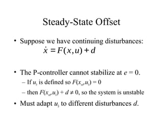
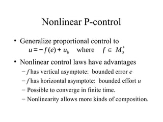
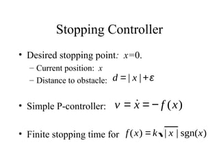
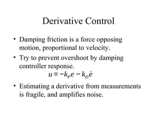
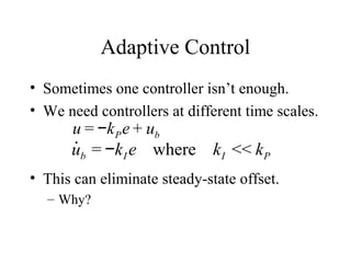
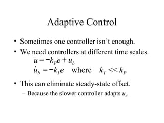
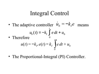
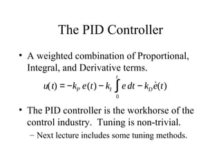
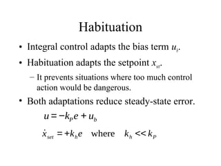
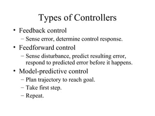
Lecture 4:
Basic Concepts in Control
CS 344R: Robotics
Benjamin Kuipers
Controlling a Simple System
• Consider a simple system:
– Scalar variables x and u, not vectors x and u.
– Assume x is observable: y = G(x) = x
– Assume effect of motor command u:
• The setpoint xset is the desired value.
– The controller responds to error: e = x − xset
• The goal is to set u to reach e = 0.
˙x = F(x,u)
∂F
∂u
> 0
The intuitions behind control
• Use action u to push back toward error e = 0
• What does pushing back do?
– Velocity versus acceleration control
• How much should we push back?
– What does the magnitude of u depend on?
Velocity or acceleration control?
• Velocity:
• Acceleration:
˙x= ( ˙x) = F (x,u) = (u)
x= (x)
x=
x
v
⎛
⎝
⎜⎜
⎞
⎠
⎟⎟
˙x =
˙x
˙v
⎛
⎝
⎜⎜
⎞
⎠
⎟⎟= F (x,u) =
v
u
⎛
⎝
⎜⎜
⎞
⎠
⎟⎟
˙v = ˙˙x = u
Laws of Motion in Physics
• Newton’s Law: F=ma or a=F/m.
• But Aristotle said:
– Velocity, not acceleration, is proportional to the
force on a body.
• Who is right? Why should we care?
– (We’ll come back to this.)
˙x =
˙x
˙v
⎛
⎝
⎜
⎞
⎠
⎟=
v
F /m
⎛
⎝
⎜
⎞
⎠
⎟
The Bang-Bang Controller
• Push back, against the direction of the error
• Error:
• To prevent chatter around
• Household thermostat. Not very subtle.
e = x − xset
e < 0 ⇒ u := on ⇒ ˙x = F (x,on) > 0
e > 0 ⇒ u := off ⇒ ˙x = F (x,off ) < 0
e < −ε ⇒ u := on
e > +ε ⇒ u := off
e = 0
Proportional Control
• Push back, proportional to the error.
– Set ub so that
• For a linear system, exponential
convergence.
• The controller gain k determines how
quickly the system responds to error.
u = −ke + ub
˙x = F(xset ,ub ) = 0
x(t) = Ce
−α t
+ xset
Velocity Control
• You want the robot to move at velocity vset.
• You command velocity vcmd.
• You observe velocity vobs.
• Define a first-order controller:
– k is the controller gain.
˙vcmd = −k(vobs − vset )
Steady-State Offset
• Suppose we have continuing disturbances:
• The P-controller cannot stabilize at e = 0.
– Why not?
˙x = F(x,u) + d
Steady-State Offset
• Suppose we have continuing disturbances:
• The P-controller cannot stabilize at e = 0.
– If ub is defined so F(xset,ub) = 0
– then F(xset,ub) + d ≠ 0, so the system is unstable
• Must adapt ub to different disturbances d.
˙x = F(x,u) + d
Nonlinear P-control
• Generalize proportional control to
• Nonlinear control laws have advantages
– f has vertical asymptote: bounded error e
– f has horizontal asymptote: bounded effort u
– Possible to converge in finite time.
– Nonlinearity allows more kinds of composition.
u = − f (e) + ub where f ∈ M0
+
Stopping Controller
• Desired stopping point: x=0.
– Current position: x
– Distance to obstacle:
• Simple P-controller:
• Finite stopping time for
d = | x |+ε
v = ˙x = − f (x)
f(x) = k | x | sgn(x)
Derivative Control
• Damping friction is a force opposing
motion, proportional to velocity.
• Try to prevent overshoot by damping
controller response.
• Estimating a derivative from measurements
is fragile, and amplifies noise.
u = −kPe − kD
˙e
Adaptive Control
• Sometimes one controller isn’t enough.
• We need controllers at different time scales.
• This can eliminate steady-state offset.
– Why?
u = −kPe + ub
˙ub = −kI e where kI << kP
Adaptive Control
• Sometimes one controller isn’t enough.
• We need controllers at different time scales.
• This can eliminate steady-state offset.
– Because the slower controller adapts ub.
u = −kPe + ub
˙ub = −kI e where kI << kP
Integral Control
• The adaptive controller means
• Therefore
• The Proportional-Integral (PI) Controller.
˙ub = −kI e
ub (t) = −kI e dt
0
t
∫ + ub
u(t) = −kP e(t) − kI edt
0
t
∫ + ub
The PID Controller
• A weighted combination of Proportional,
Integral, and Derivative terms.
• The PID controller is the workhorse of the
control industry. Tuning is non-trivial.
– Next lecture includes some tuning methods.
u(t) = −kP e(t) − kI e dt
0
t
∫ − kD
˙e(t)
Habituation
• Integral control adapts the bias term ub.
• Habituation adapts the setpoint xset.
– It prevents situations where too much control
action would be dangerous.
• Both adaptations reduce steady-state error.
u = −kPe + ub
˙xset = +khe where kh << kP
Types of Controllers
• Feedback control
– Sense error, determine control response.
• Feedforward control
– Sense disturbance, predict resulting error,
respond to predicted error before it happens.
• Model-predictive control
– Plan trajectory to reach goal.
– Take first step.
– Repeat.
Laws of Motion in Physics
• Newton’s Law: F=ma or a=F/m.
• But Aristotle said:
– Velocity, not acceleration, is proportional to the
force on a body.
• Who is right? Why should we care?
˙x =
˙x
˙v
⎛
⎝
⎜
⎞
⎠
⎟=
v
F /m
⎛
⎝
⎜
⎞
⎠
⎟
Who is right? Aristotle!
• Try it! It takes constant force to keep an
object moving at constant velocity.
– Ignore brief transients
• Aristotle was a genius to recognize that
there could be laws of motion, and to
formulate a useful and accurate one.
• This law is true because our everyday world
is friction-dominated.
Who is right? Newton!
• Newton’s genius was to recognize that the
true laws of motion may be different from
what we usually observe on earth.
• For the planets, without friction, motion
continues without force.
• For Aristotle, “force” means Fexternal.
• For Newton, “force” means Ftotal.
– On Earth, you must include Ffriction.
From Newton back to Aristotle
• Ftotal = Fexternal + Ffriction
• Ffriction = −f(v) for some monotonic f.
• Thus:
• Velocity v moves quickly to equilibrium:
• Terminal velocity vfinal depends on:
– Fext, m, and the friction function f(v).
– So Aristotle was right! In a friction-dominated
world.
˙x
˙v
⎛
⎝
⎜
⎞
⎠
⎟=
v
F /m
⎛
⎝
⎜
⎞
⎠
⎟=
v
1
m Fext − 1
m f (v)
⎛
⎝
⎜
⎞
⎠
⎟
˙v = 1
m
Fext − 1
m
f (v)

Week10 ben-control

  • 1.
    Lecture 4: Basic Conceptsin Control CS 344R: Robotics Benjamin Kuipers
  • 2.
    Controlling a SimpleSystem • Consider a simple system: – Scalar variables x and u, not vectors x and u. – Assume x is observable: y = G(x) = x – Assume effect of motor command u: • The setpoint xset is the desired value. – The controller responds to error: e = x − xset • The goal is to set u to reach e = 0. ˙x = F(x,u) ∂F ∂u > 0
  • 3.
    The intuitions behindcontrol • Use action u to push back toward error e = 0 • What does pushing back do? – Velocity versus acceleration control • How much should we push back? – What does the magnitude of u depend on?
  • 4.
    Velocity or accelerationcontrol? • Velocity: • Acceleration: ˙x= ( ˙x) = F (x,u) = (u) x= (x) x= x v ⎛ ⎝ ⎜⎜ ⎞ ⎠ ⎟⎟ ˙x = ˙x ˙v ⎛ ⎝ ⎜⎜ ⎞ ⎠ ⎟⎟= F (x,u) = v u ⎛ ⎝ ⎜⎜ ⎞ ⎠ ⎟⎟ ˙v = ˙˙x = u
  • 5.
    Laws of Motionin Physics • Newton’s Law: F=ma or a=F/m. • But Aristotle said: – Velocity, not acceleration, is proportional to the force on a body. • Who is right? Why should we care? – (We’ll come back to this.) ˙x = ˙x ˙v ⎛ ⎝ ⎜ ⎞ ⎠ ⎟= v F /m ⎛ ⎝ ⎜ ⎞ ⎠ ⎟
  • 6.
    The Bang-Bang Controller •Push back, against the direction of the error • Error: • To prevent chatter around • Household thermostat. Not very subtle. e = x − xset e < 0 ⇒ u := on ⇒ ˙x = F (x,on) > 0 e > 0 ⇒ u := off ⇒ ˙x = F (x,off ) < 0 e < −ε ⇒ u := on e > +ε ⇒ u := off e = 0
  • 7.
    Proportional Control • Pushback, proportional to the error. – Set ub so that • For a linear system, exponential convergence. • The controller gain k determines how quickly the system responds to error. u = −ke + ub ˙x = F(xset ,ub ) = 0 x(t) = Ce −α t + xset
  • 8.
    Velocity Control • Youwant the robot to move at velocity vset. • You command velocity vcmd. • You observe velocity vobs. • Define a first-order controller: – k is the controller gain. ˙vcmd = −k(vobs − vset )
  • 9.
    Steady-State Offset • Supposewe have continuing disturbances: • The P-controller cannot stabilize at e = 0. – Why not? ˙x = F(x,u) + d
  • 10.
    Steady-State Offset • Supposewe have continuing disturbances: • The P-controller cannot stabilize at e = 0. – If ub is defined so F(xset,ub) = 0 – then F(xset,ub) + d ≠ 0, so the system is unstable • Must adapt ub to different disturbances d. ˙x = F(x,u) + d
  • 11.
    Nonlinear P-control • Generalizeproportional control to • Nonlinear control laws have advantages – f has vertical asymptote: bounded error e – f has horizontal asymptote: bounded effort u – Possible to converge in finite time. – Nonlinearity allows more kinds of composition. u = − f (e) + ub where f ∈ M0 +
  • 12.
    Stopping Controller • Desiredstopping point: x=0. – Current position: x – Distance to obstacle: • Simple P-controller: • Finite stopping time for d = | x |+ε v = ˙x = − f (x) f(x) = k | x | sgn(x)
  • 13.
    Derivative Control • Dampingfriction is a force opposing motion, proportional to velocity. • Try to prevent overshoot by damping controller response. • Estimating a derivative from measurements is fragile, and amplifies noise. u = −kPe − kD ˙e
  • 14.
    Adaptive Control • Sometimesone controller isn’t enough. • We need controllers at different time scales. • This can eliminate steady-state offset. – Why? u = −kPe + ub ˙ub = −kI e where kI << kP
  • 15.
    Adaptive Control • Sometimesone controller isn’t enough. • We need controllers at different time scales. • This can eliminate steady-state offset. – Because the slower controller adapts ub. u = −kPe + ub ˙ub = −kI e where kI << kP
  • 16.
    Integral Control • Theadaptive controller means • Therefore • The Proportional-Integral (PI) Controller. ˙ub = −kI e ub (t) = −kI e dt 0 t ∫ + ub u(t) = −kP e(t) − kI edt 0 t ∫ + ub
  • 17.
    The PID Controller •A weighted combination of Proportional, Integral, and Derivative terms. • The PID controller is the workhorse of the control industry. Tuning is non-trivial. – Next lecture includes some tuning methods. u(t) = −kP e(t) − kI e dt 0 t ∫ − kD ˙e(t)
  • 18.
    Habituation • Integral controladapts the bias term ub. • Habituation adapts the setpoint xset. – It prevents situations where too much control action would be dangerous. • Both adaptations reduce steady-state error. u = −kPe + ub ˙xset = +khe where kh << kP
  • 19.
    Types of Controllers •Feedback control – Sense error, determine control response. • Feedforward control – Sense disturbance, predict resulting error, respond to predicted error before it happens. • Model-predictive control – Plan trajectory to reach goal. – Take first step. – Repeat.
  • 20.
    Laws of Motionin Physics • Newton’s Law: F=ma or a=F/m. • But Aristotle said: – Velocity, not acceleration, is proportional to the force on a body. • Who is right? Why should we care? ˙x = ˙x ˙v ⎛ ⎝ ⎜ ⎞ ⎠ ⎟= v F /m ⎛ ⎝ ⎜ ⎞ ⎠ ⎟
  • 21.
    Who is right?Aristotle! • Try it! It takes constant force to keep an object moving at constant velocity. – Ignore brief transients • Aristotle was a genius to recognize that there could be laws of motion, and to formulate a useful and accurate one. • This law is true because our everyday world is friction-dominated.
  • 22.
    Who is right?Newton! • Newton’s genius was to recognize that the true laws of motion may be different from what we usually observe on earth. • For the planets, without friction, motion continues without force. • For Aristotle, “force” means Fexternal. • For Newton, “force” means Ftotal. – On Earth, you must include Ffriction.
  • 23.
    From Newton backto Aristotle • Ftotal = Fexternal + Ffriction • Ffriction = −f(v) for some monotonic f. • Thus: • Velocity v moves quickly to equilibrium: • Terminal velocity vfinal depends on: – Fext, m, and the friction function f(v). – So Aristotle was right! In a friction-dominated world. ˙x ˙v ⎛ ⎝ ⎜ ⎞ ⎠ ⎟= v F /m ⎛ ⎝ ⎜ ⎞ ⎠ ⎟= v 1 m Fext − 1 m f (v) ⎛ ⎝ ⎜ ⎞ ⎠ ⎟ ˙v = 1 m Fext − 1 m f (v)

Editor's Notes

  • #3 Check how many people are lost after the first bullet.