The document provides an introduction to PID control, including:
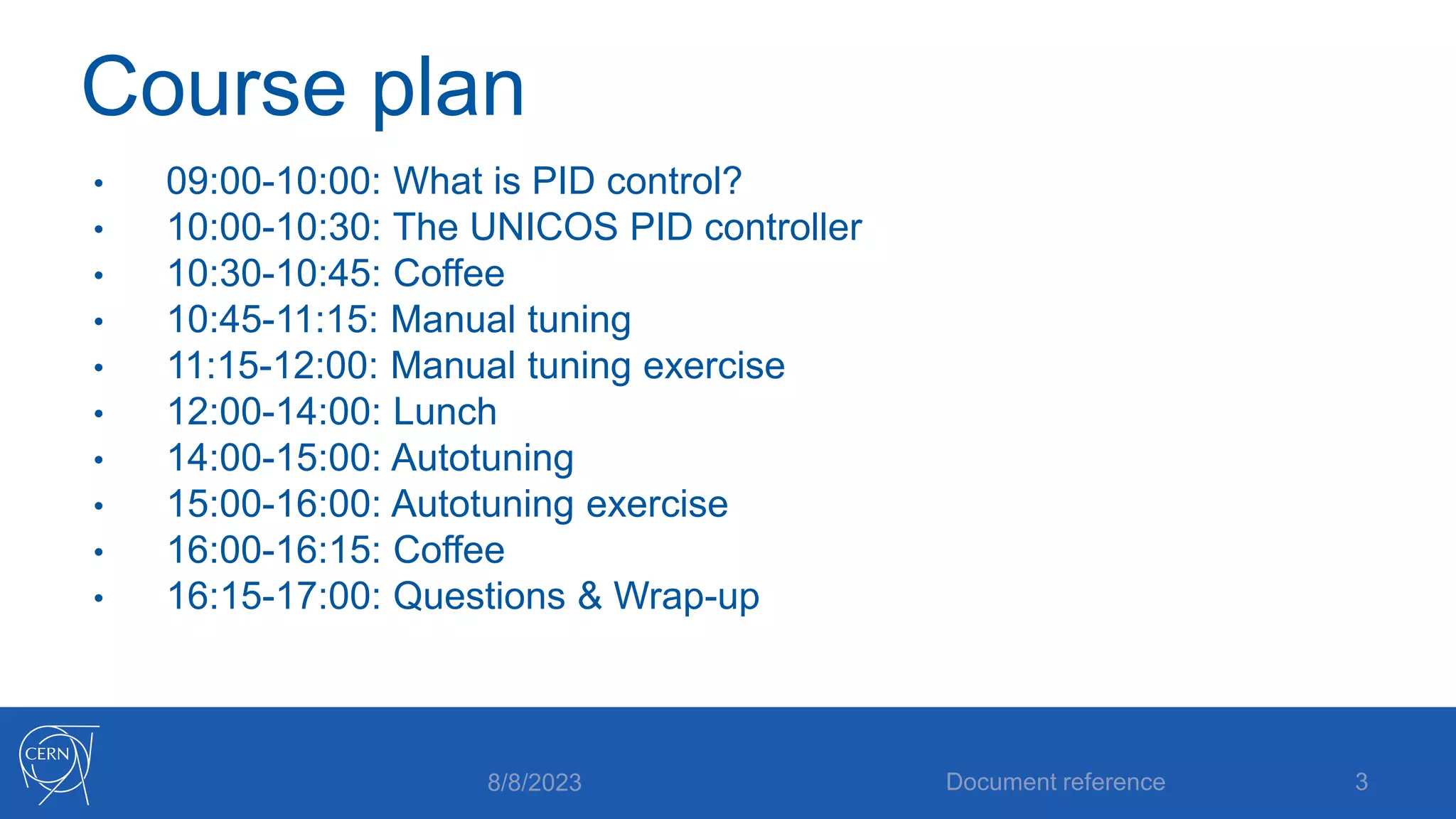
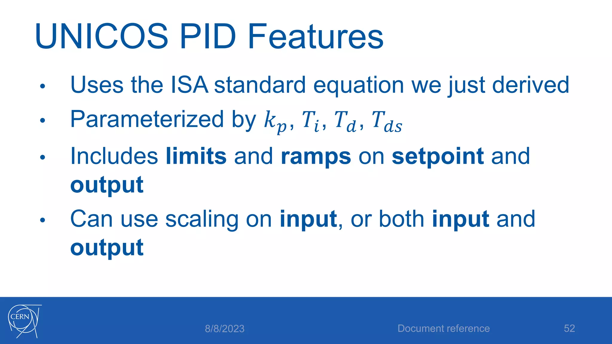
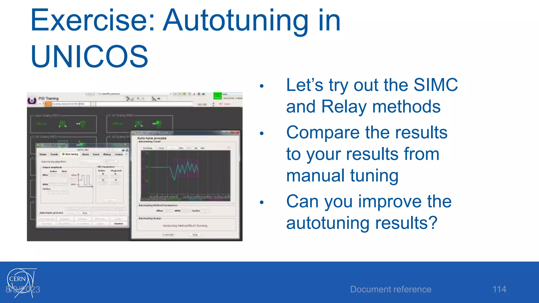
- A course plan that covers what PID control is, using the UNICOS PID controller, manual and automatic tuning exercises, and a question/wrap-up session.
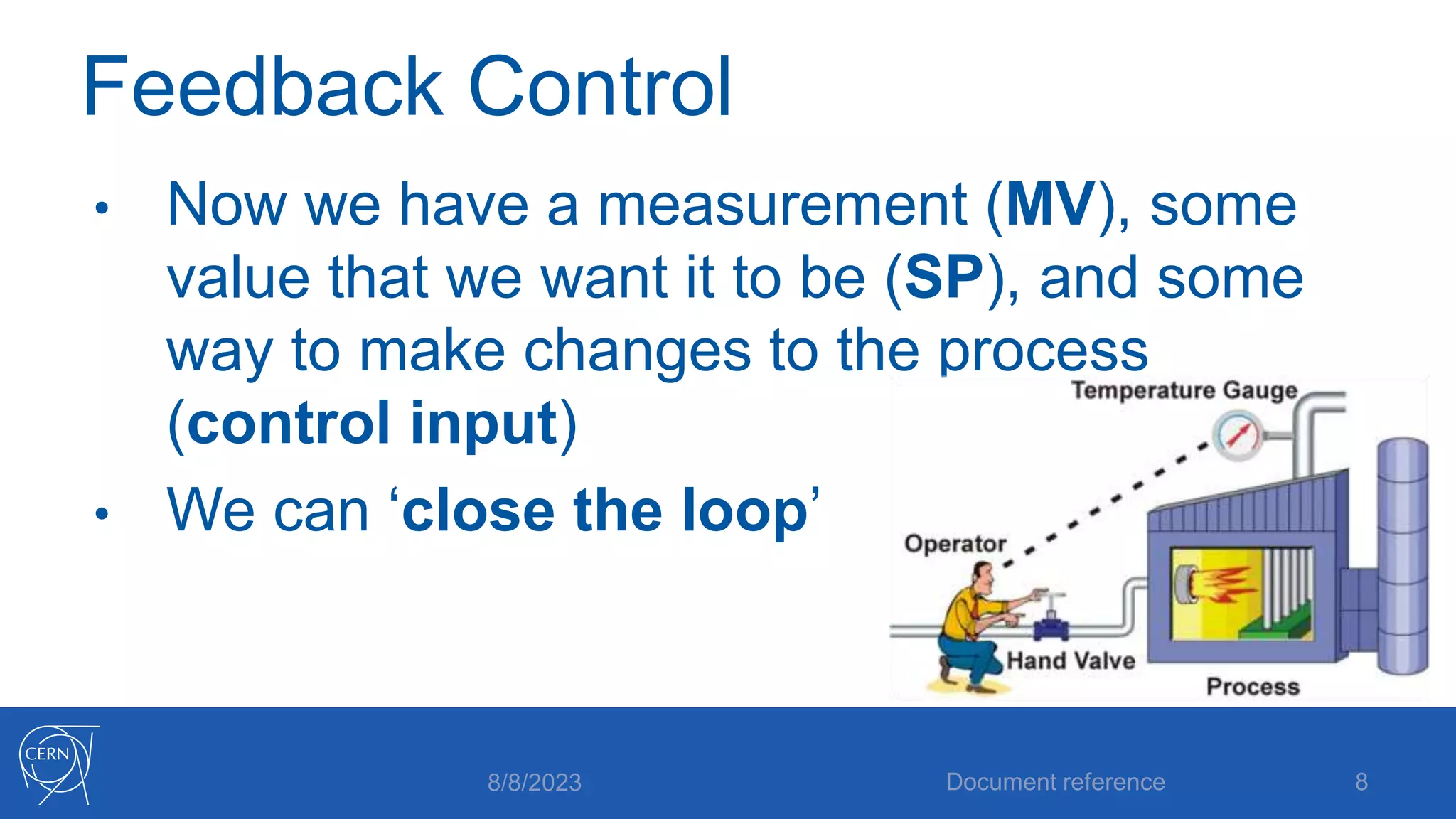
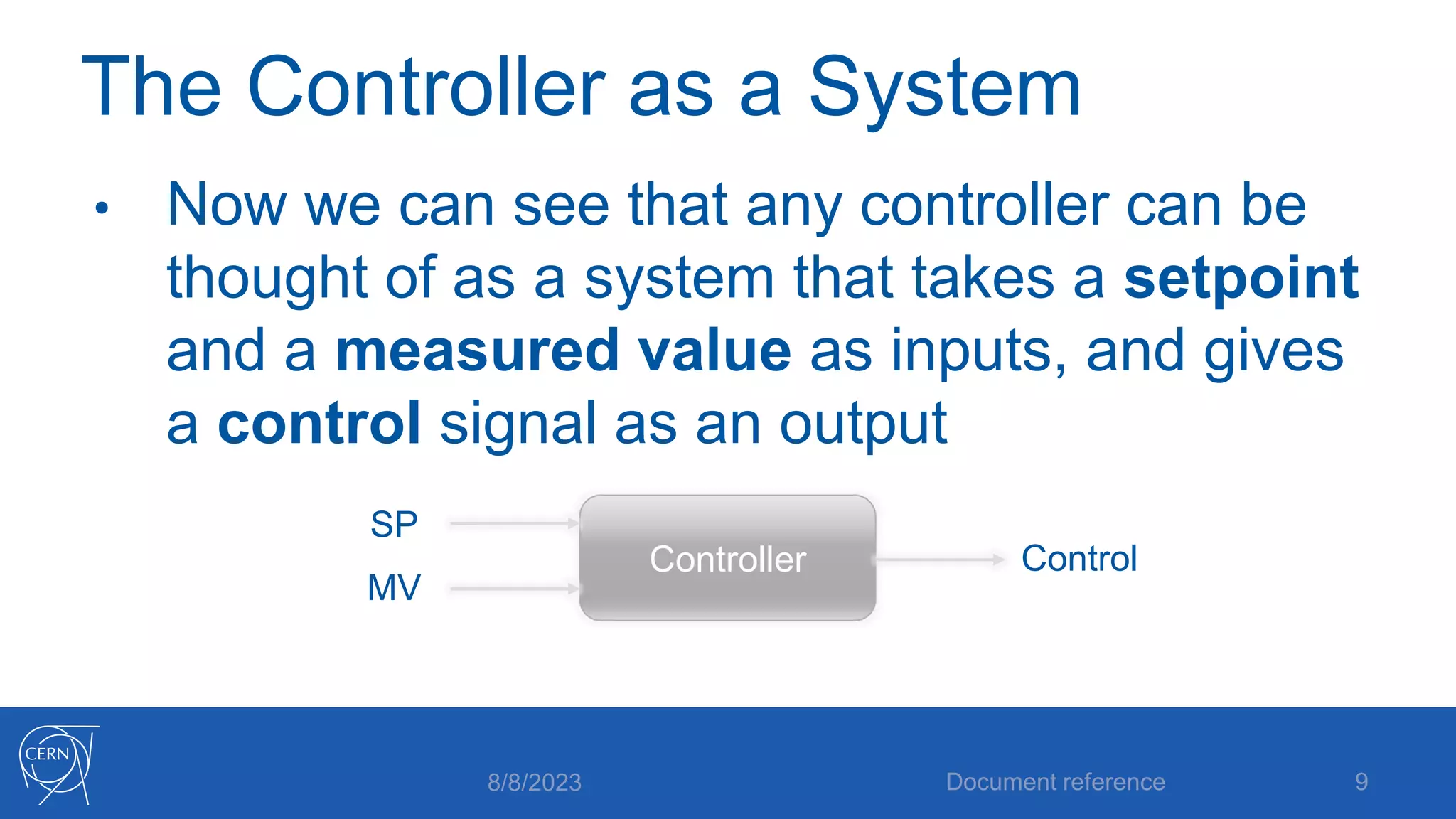
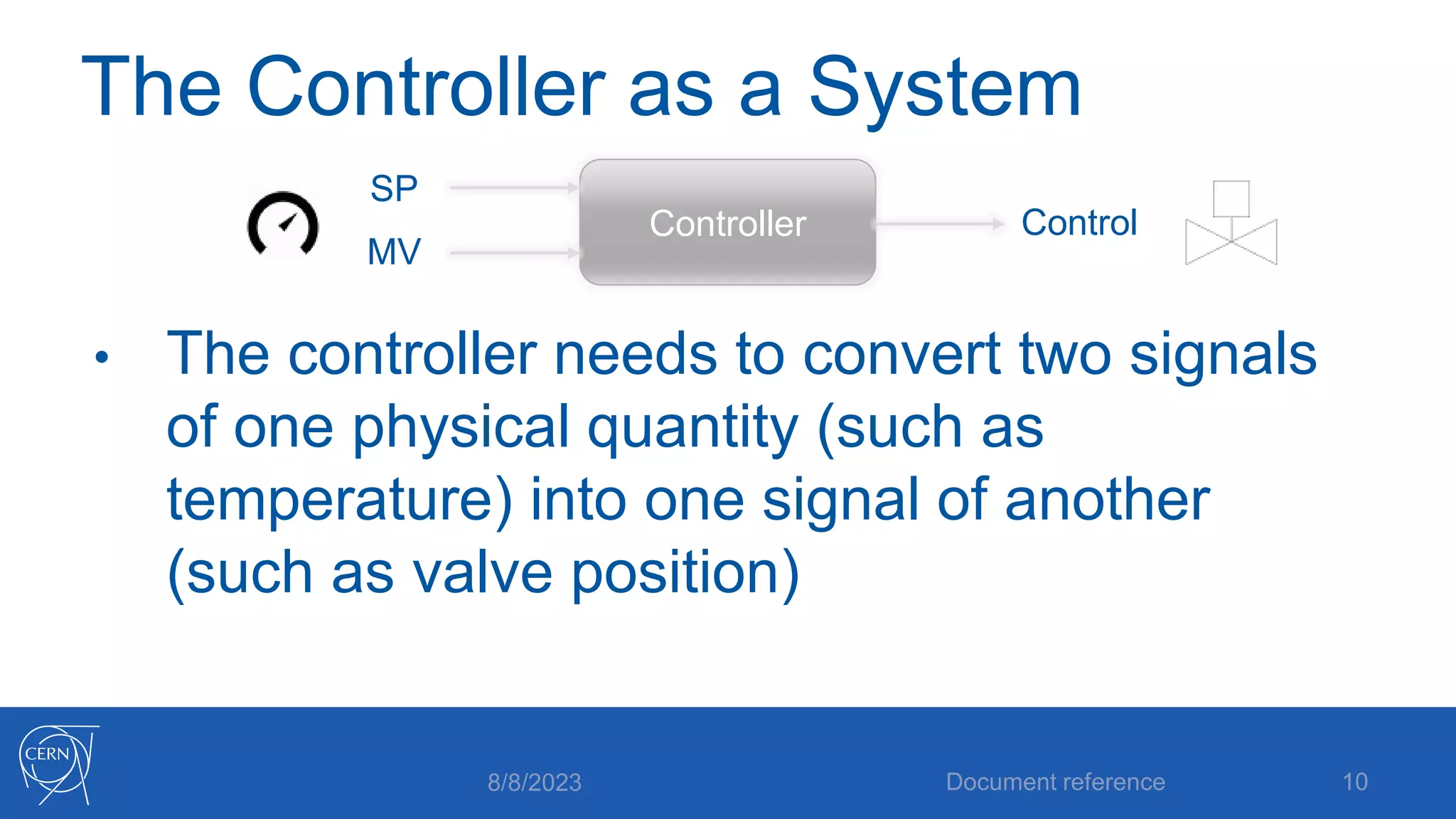
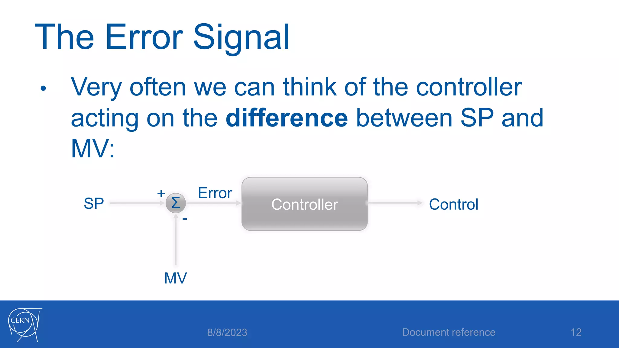
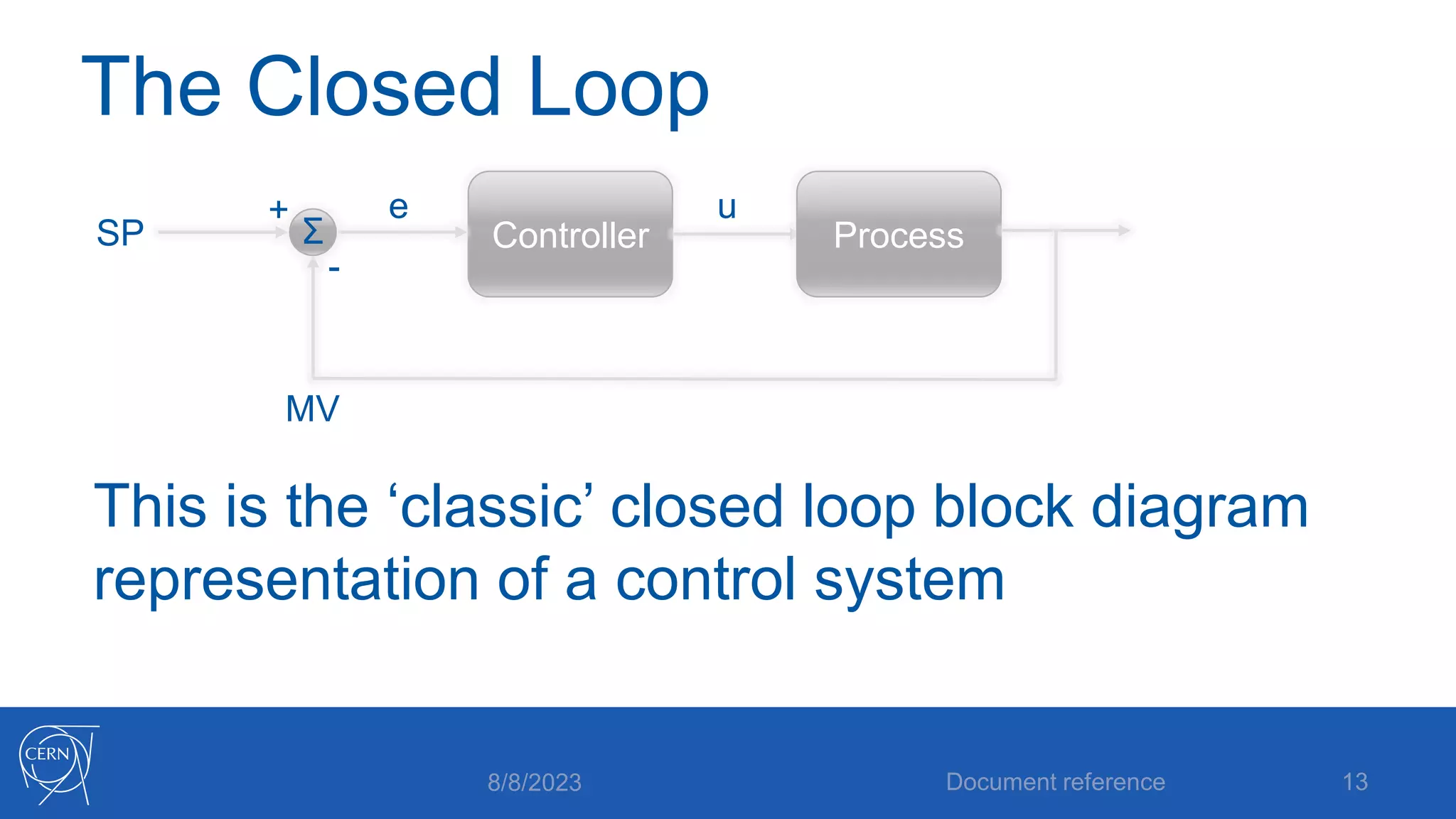
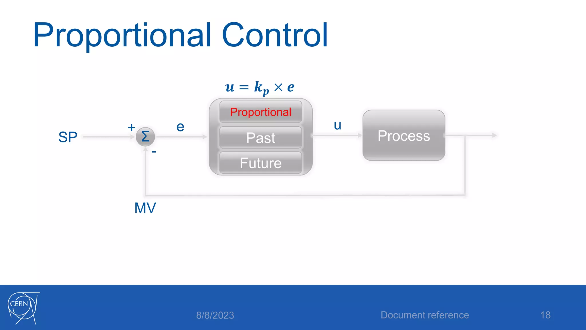
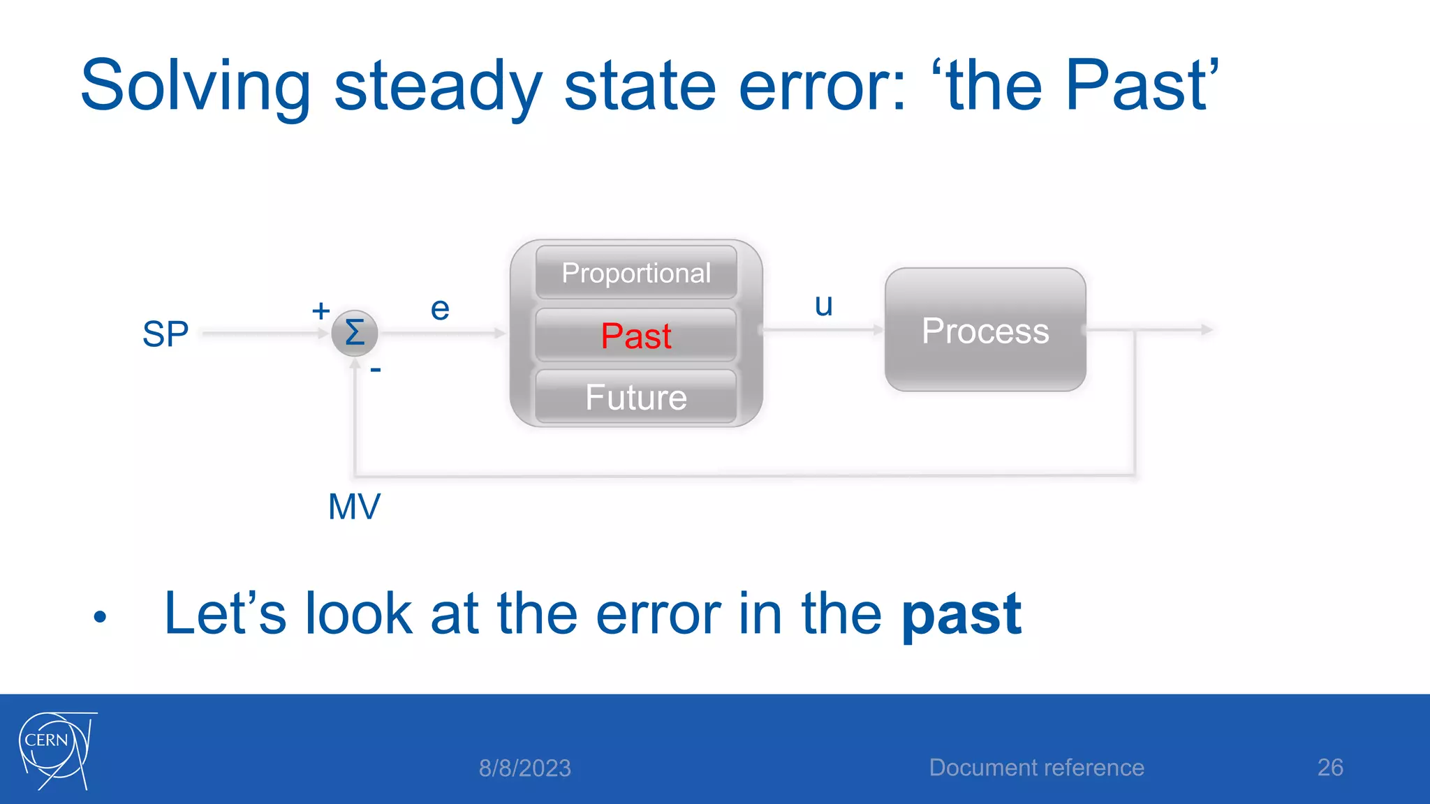
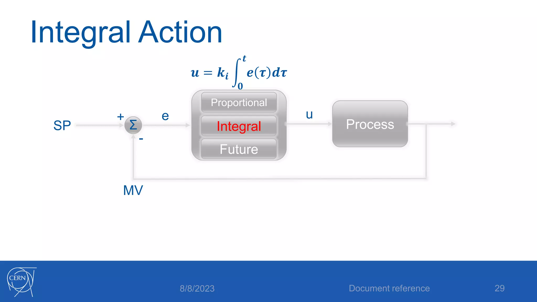
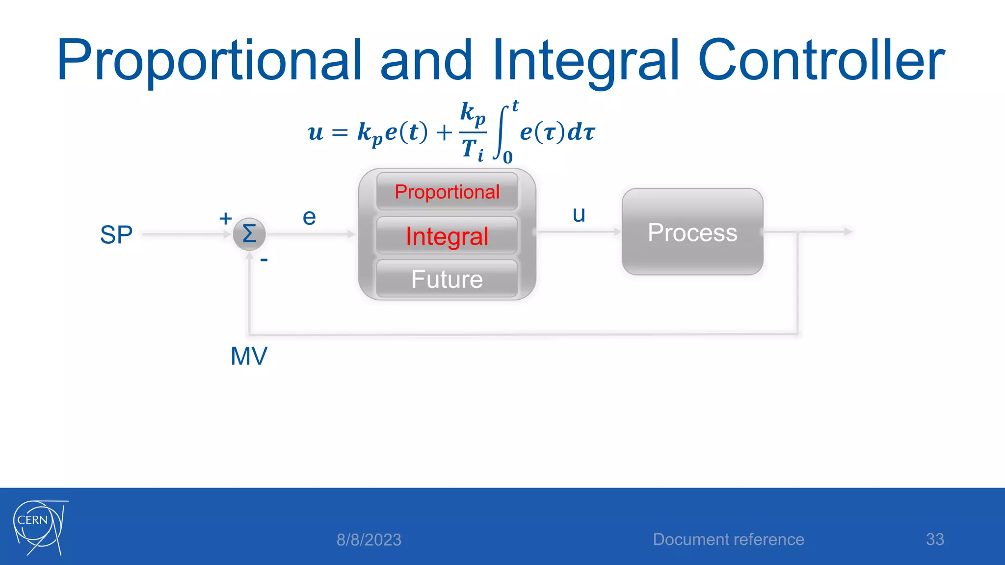
- An explanation of the components of a feedback control system including defining the setpoint, influencing and observing the process, and closing the control loop.
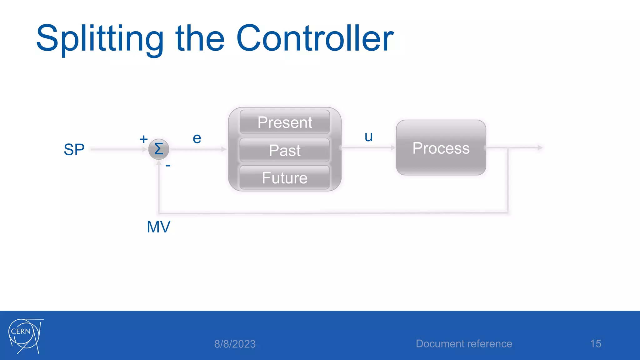
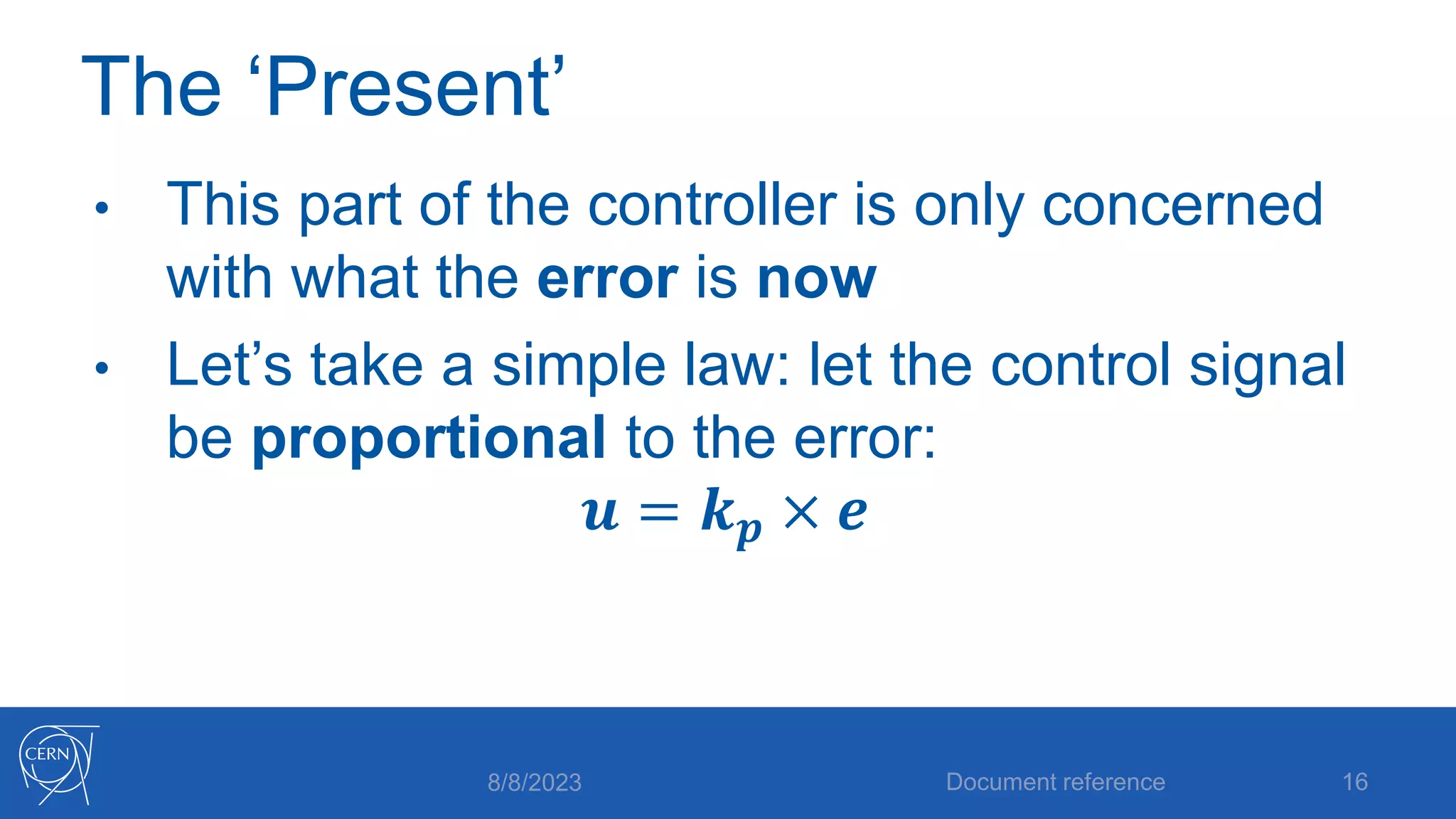
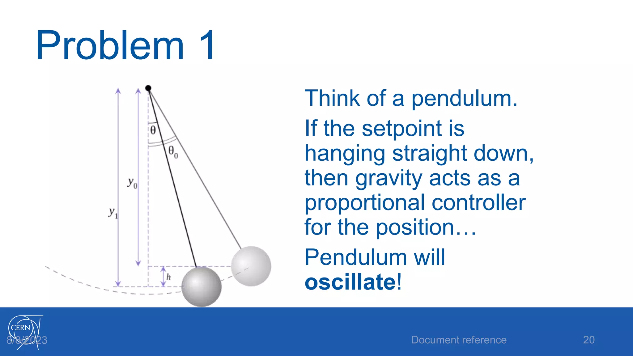
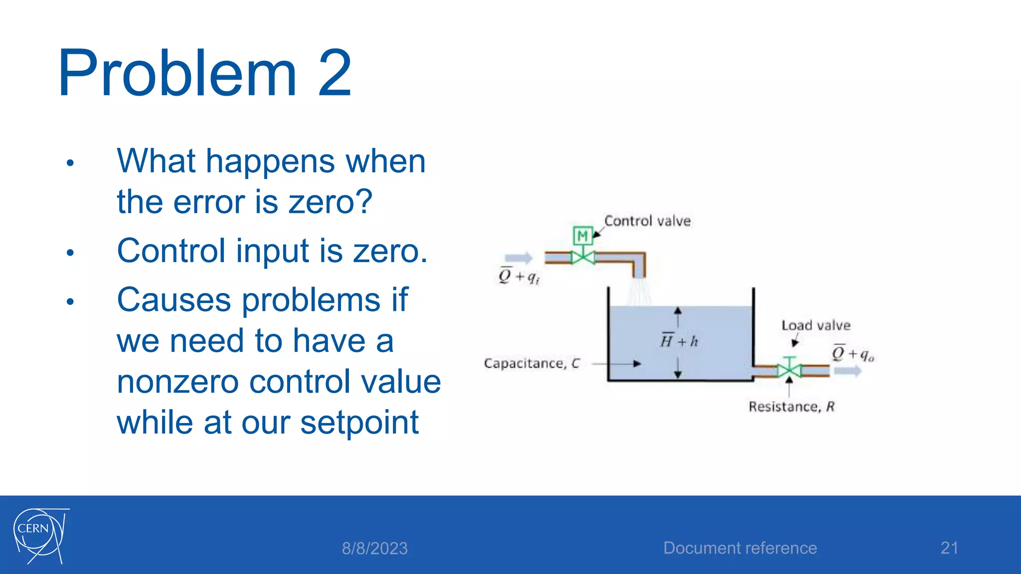
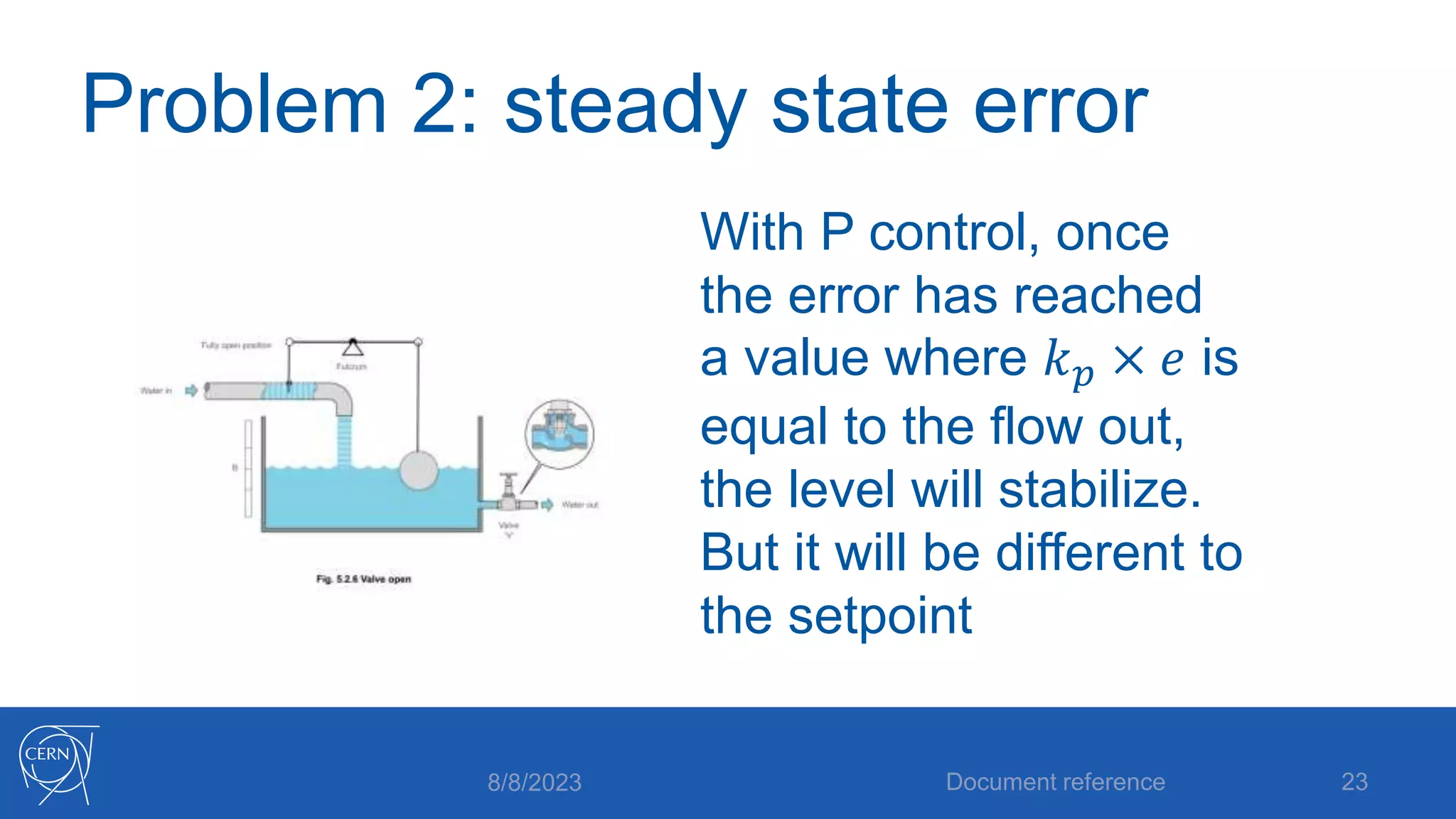
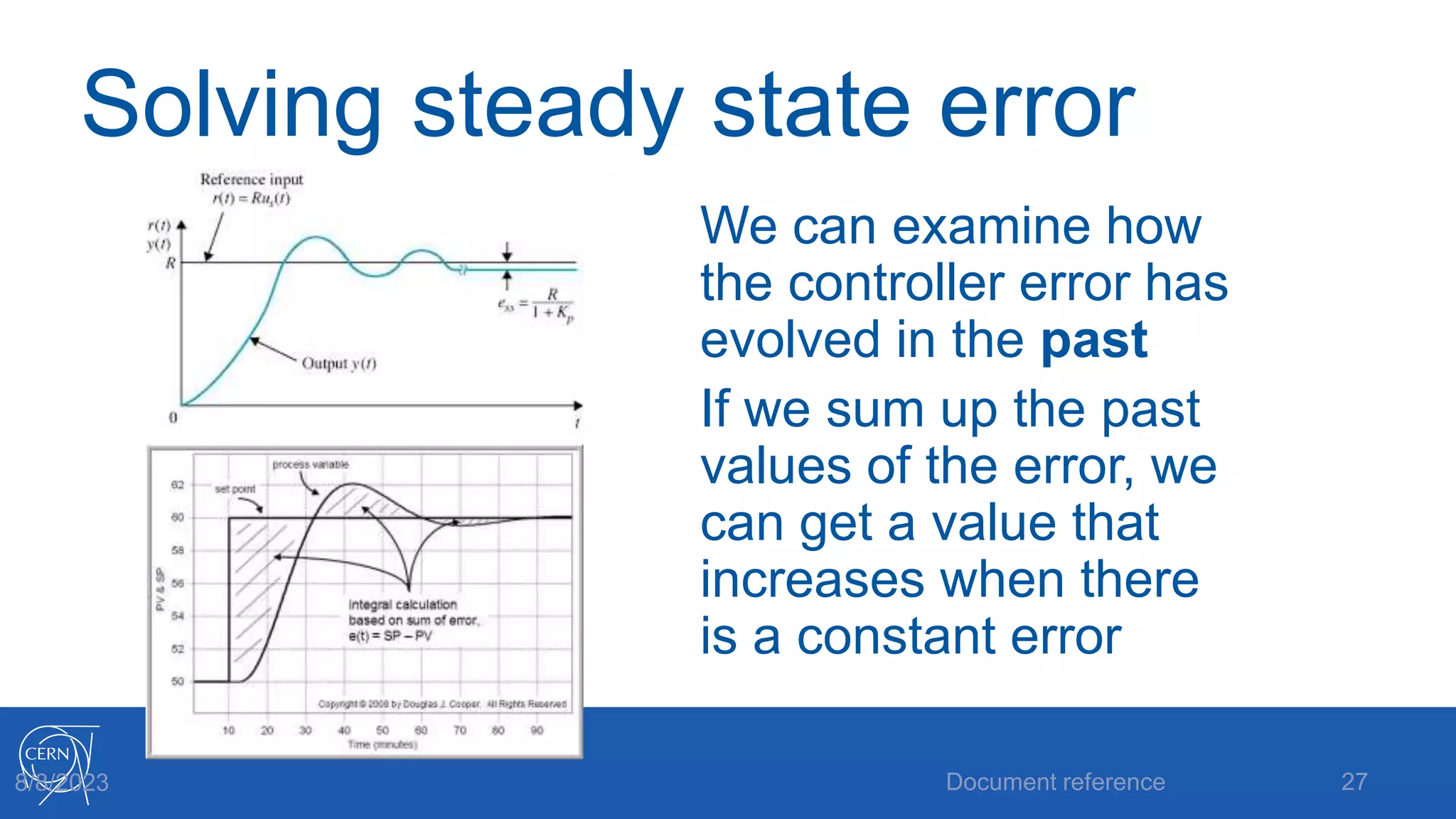
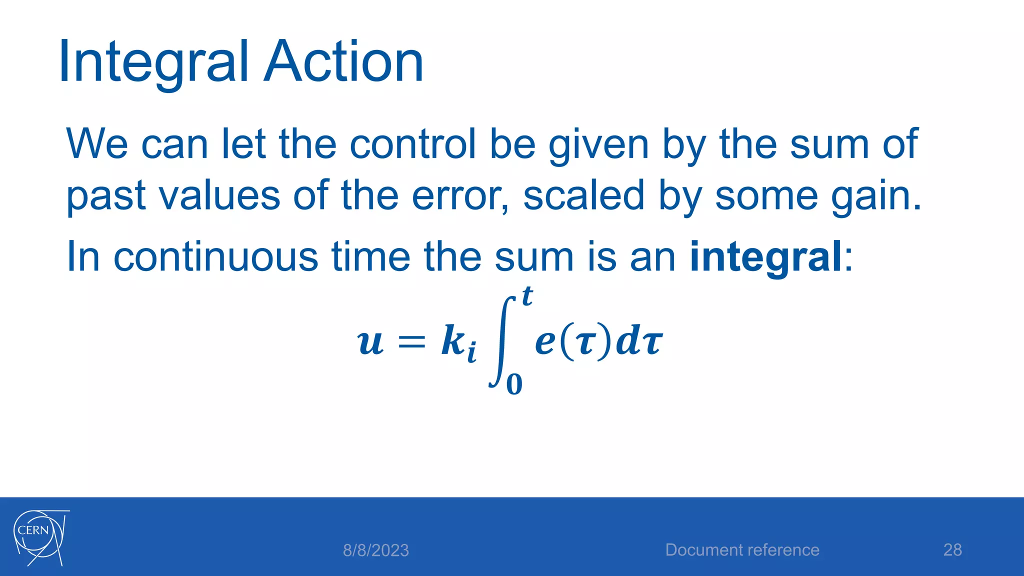
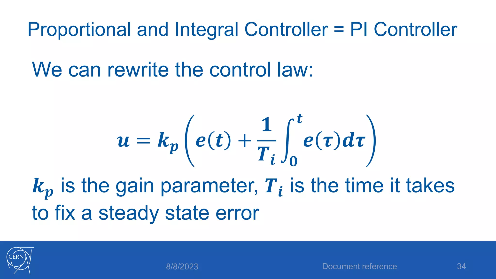
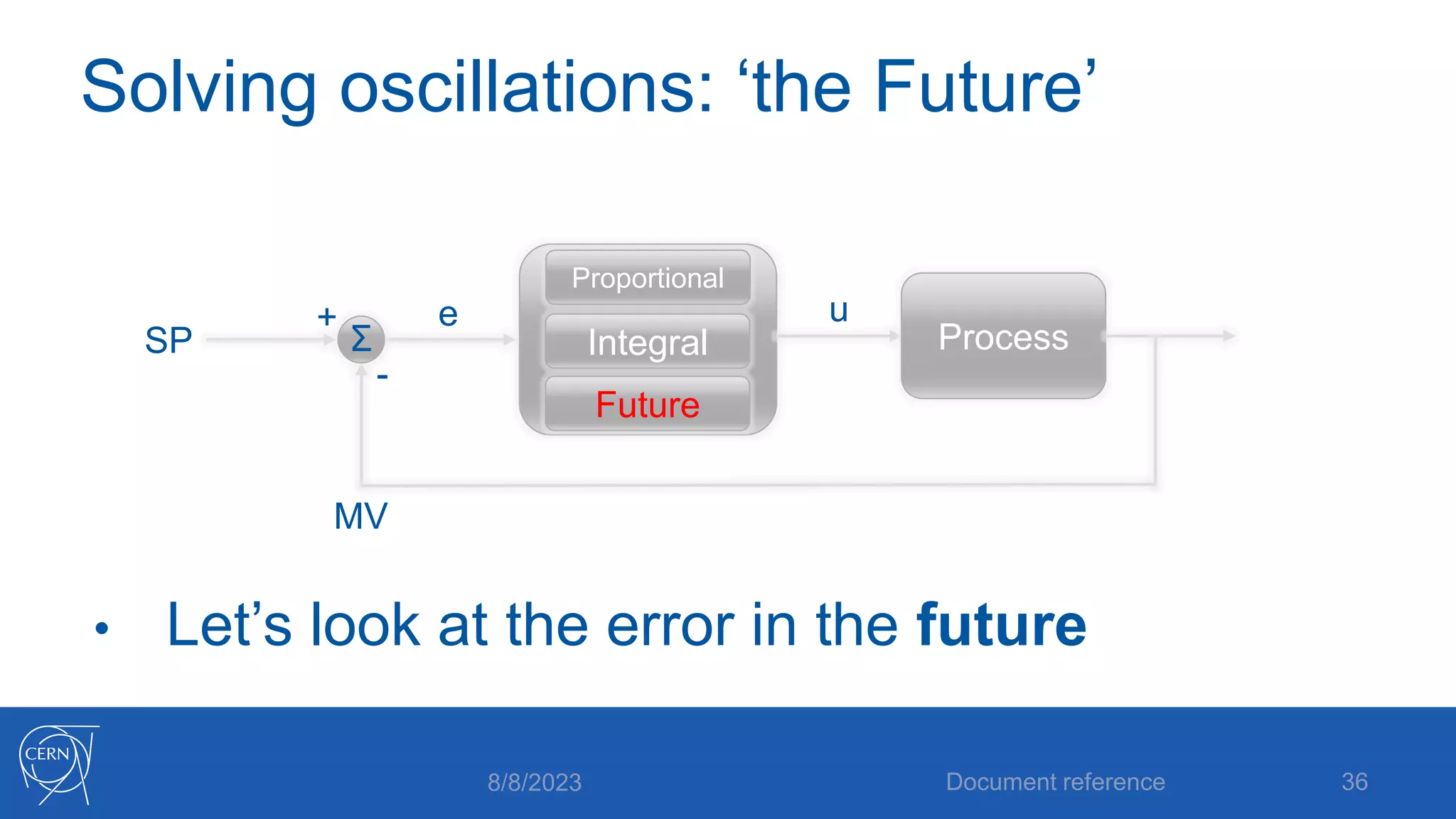
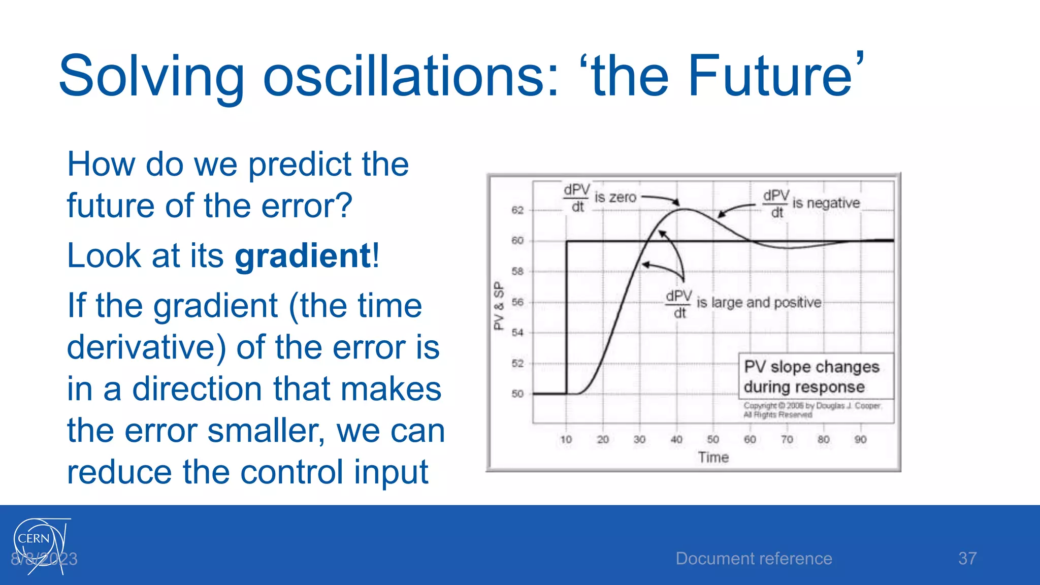
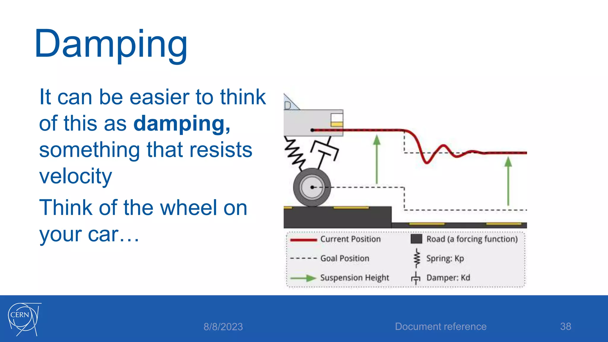
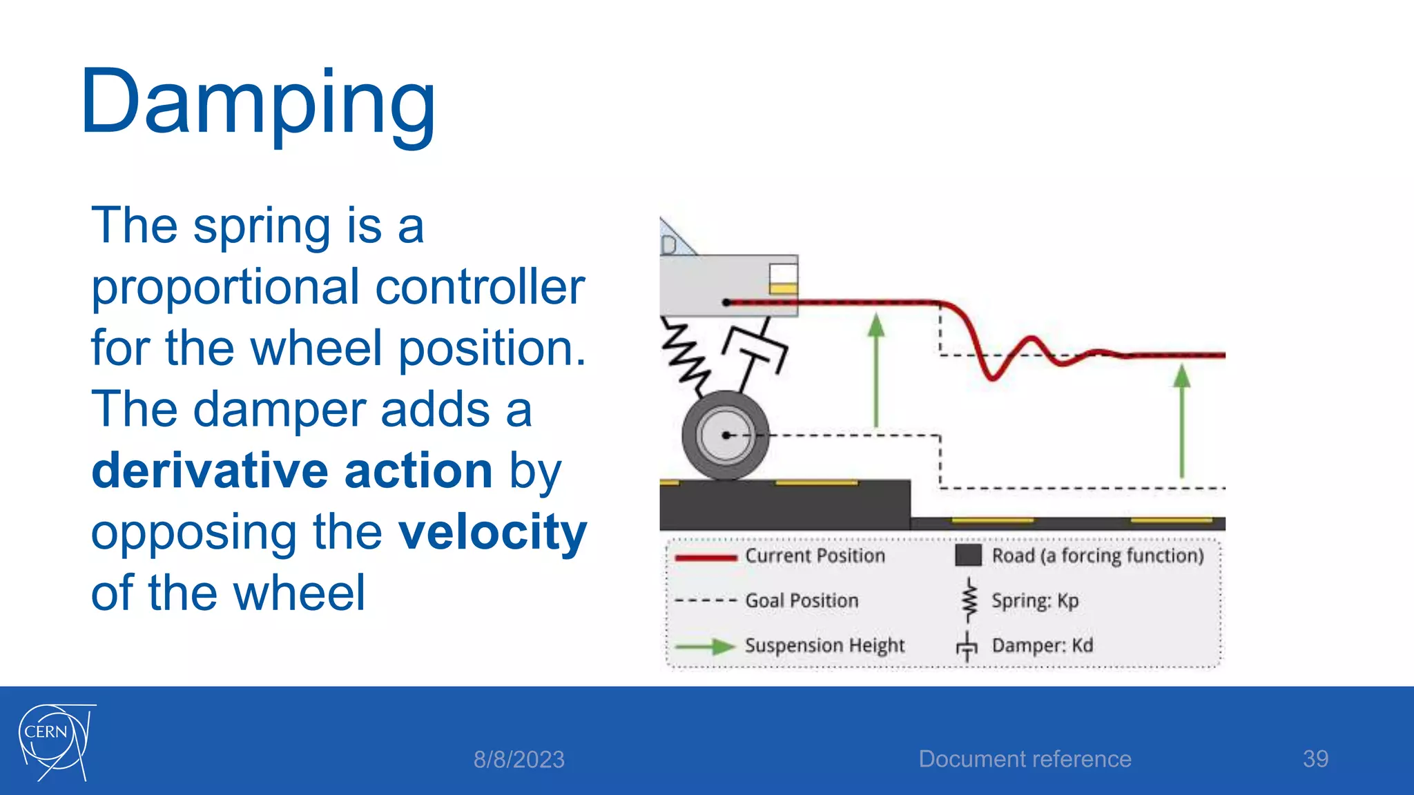
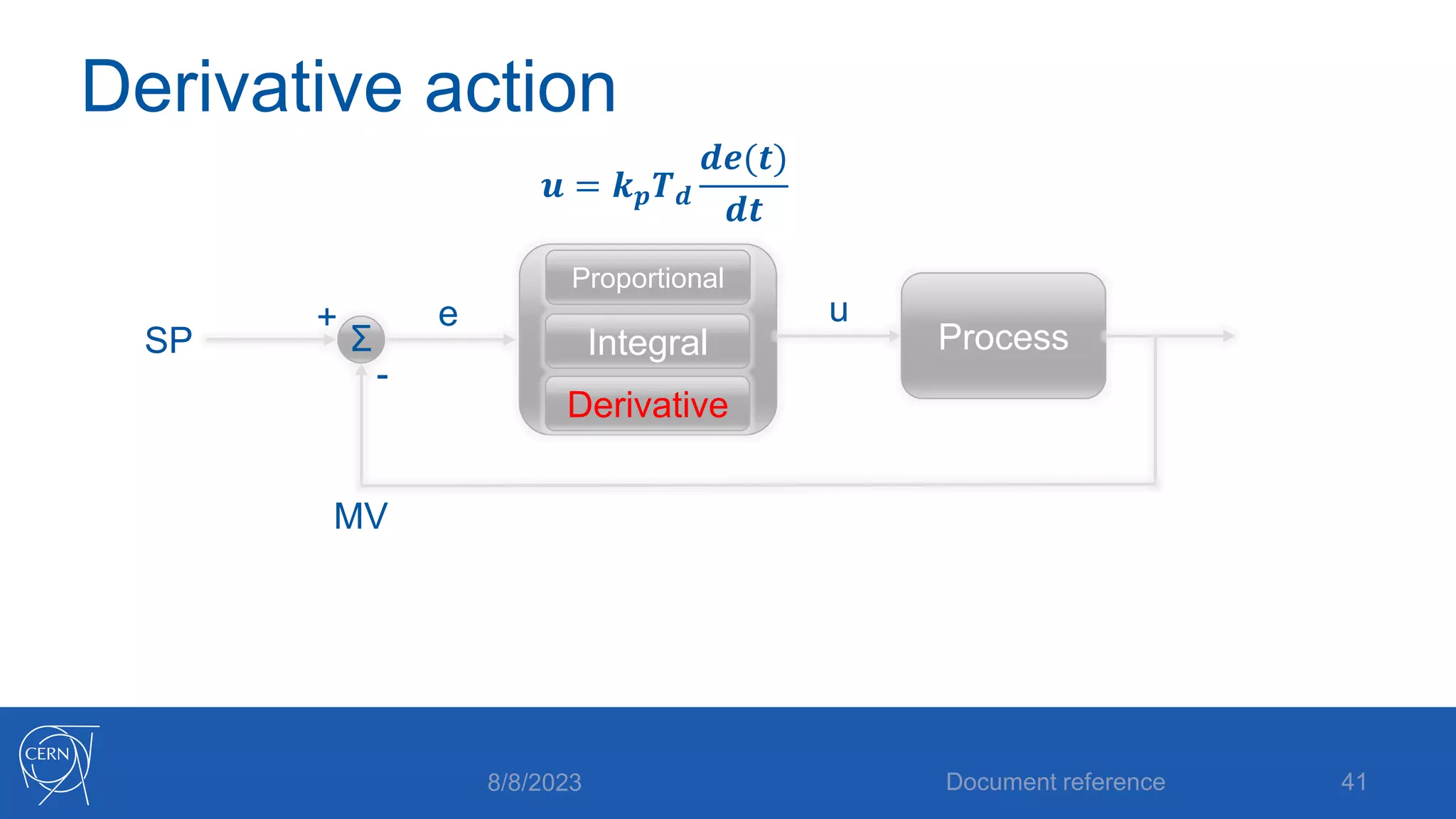
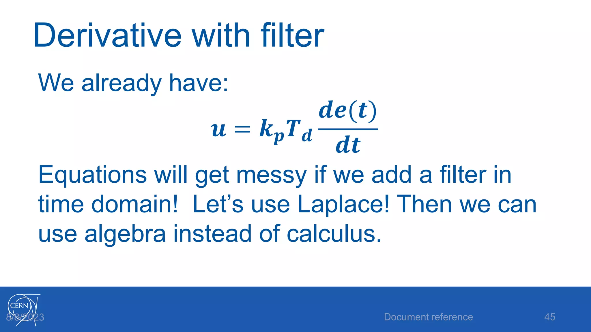
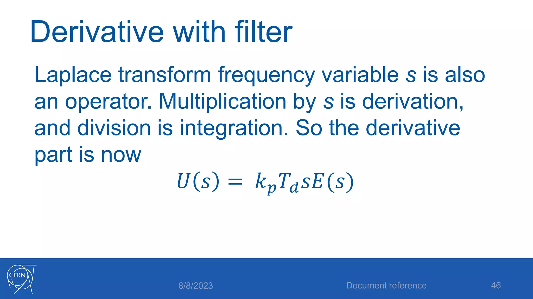
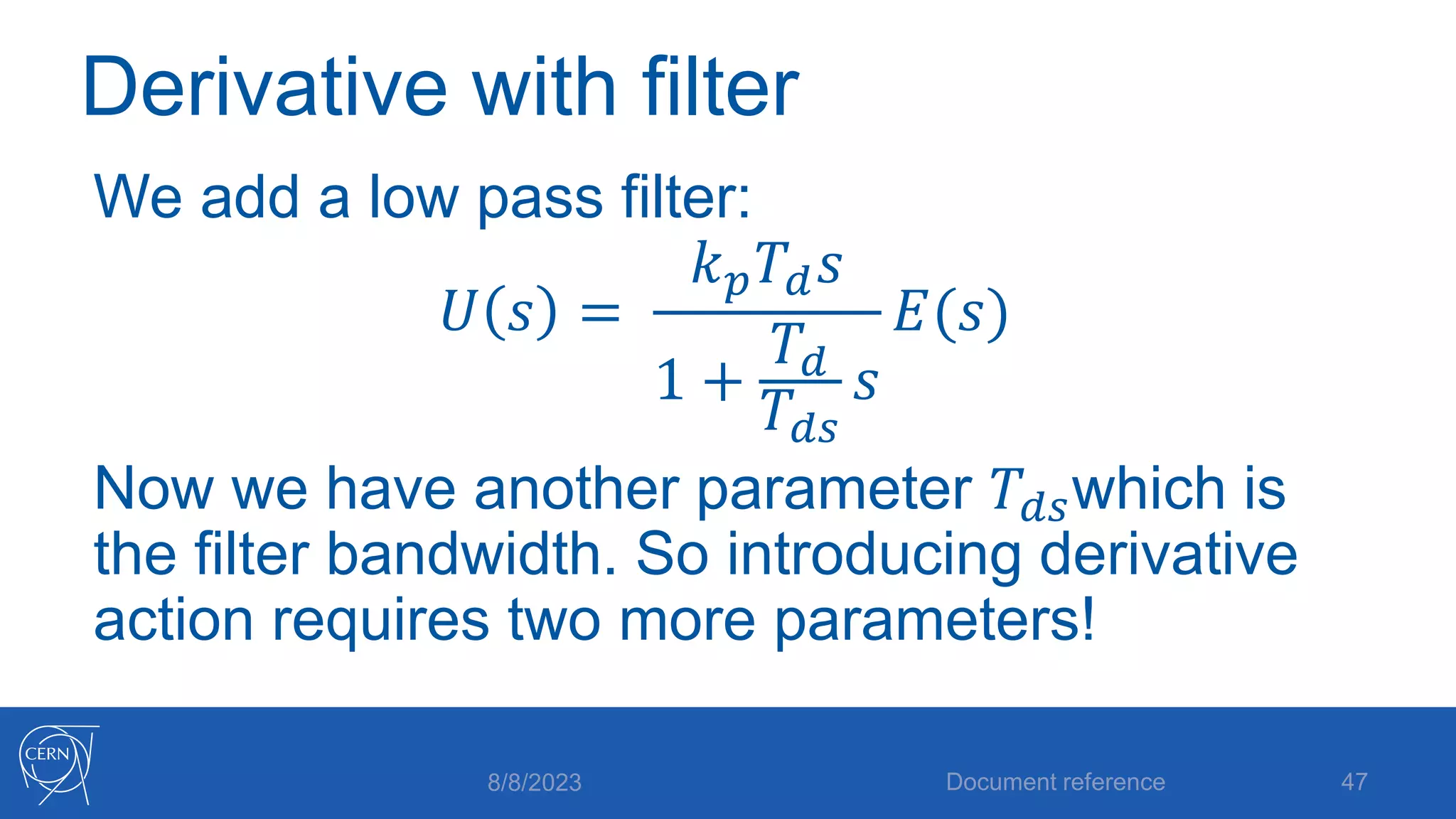
- How proportional, integral and derivative control actions work to solve the problems of steady state error and oscillations in proportional-only control.
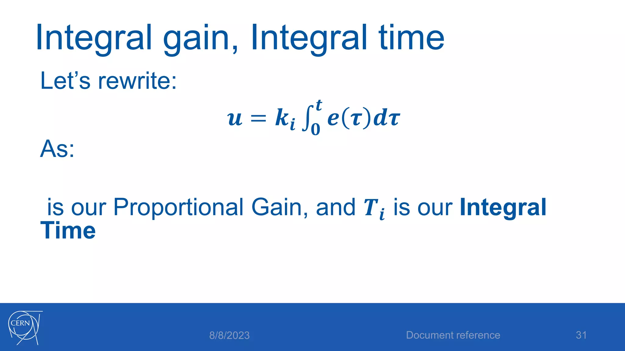
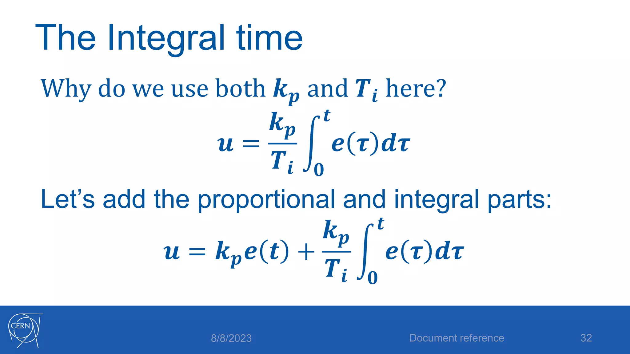
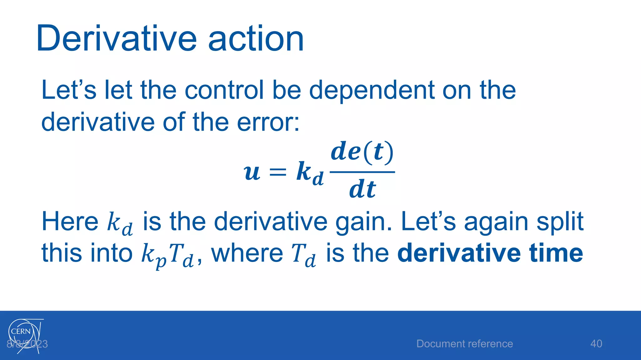
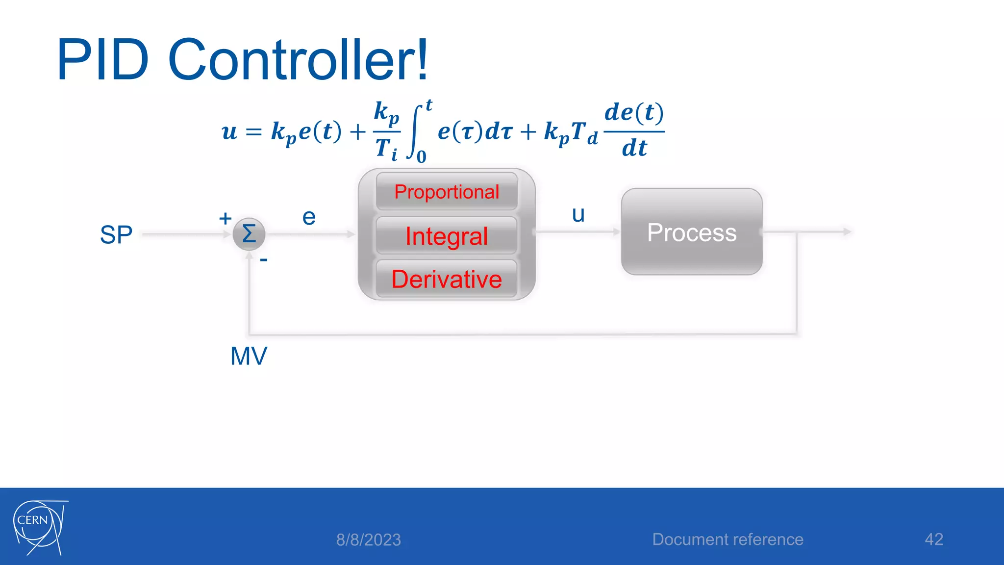
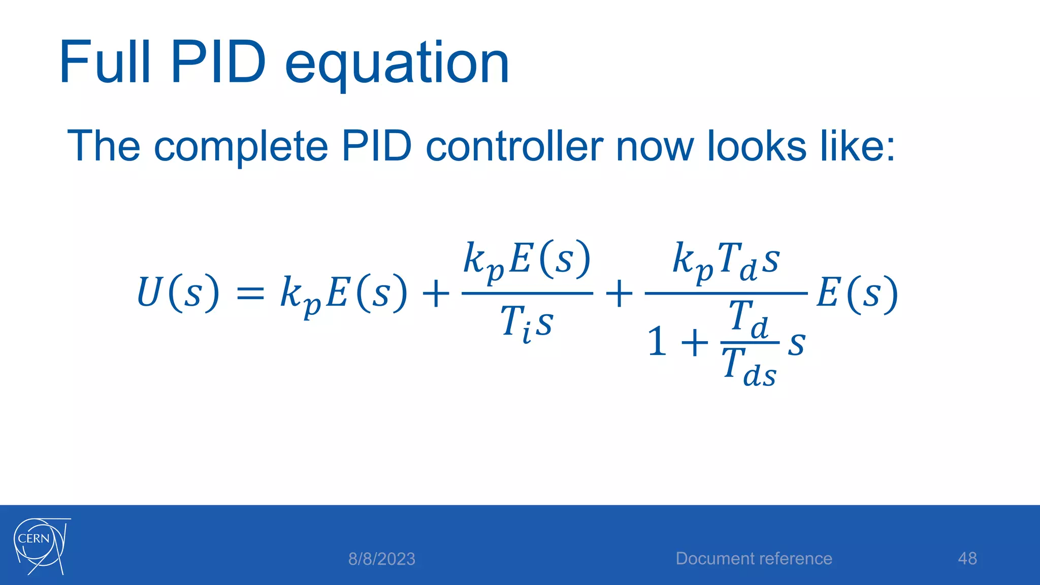
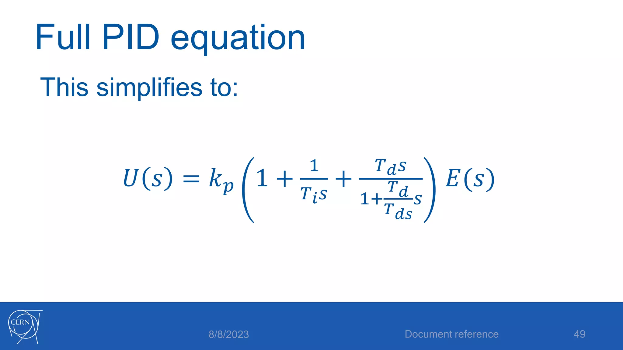
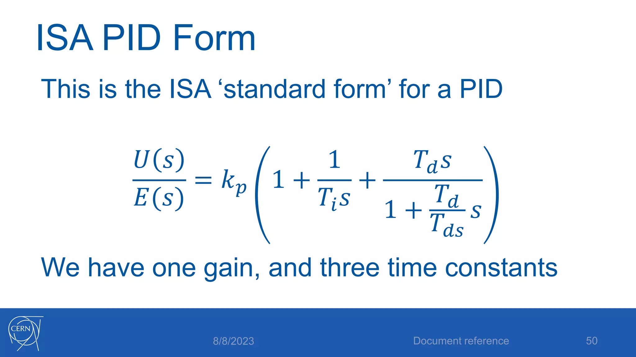
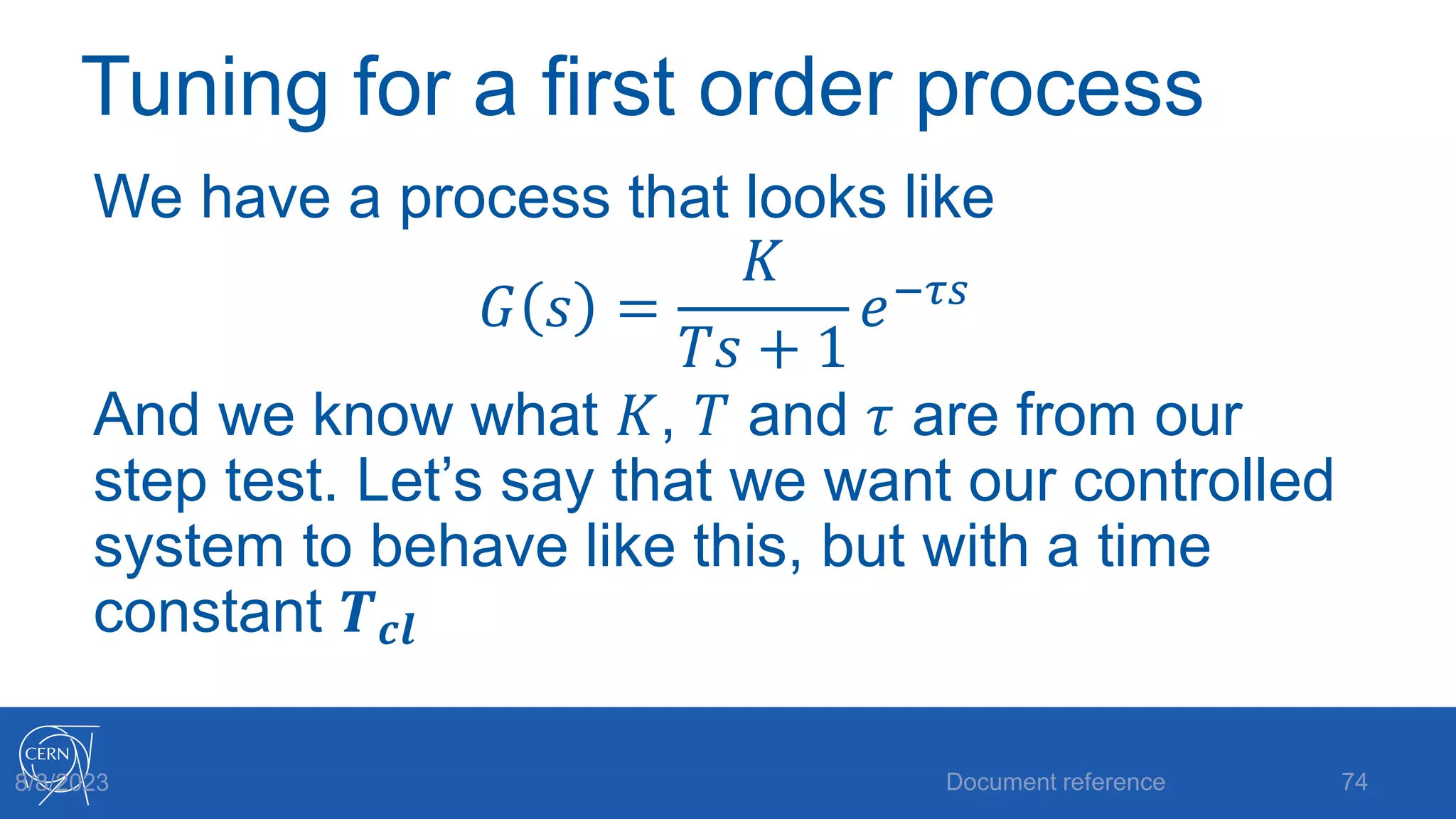
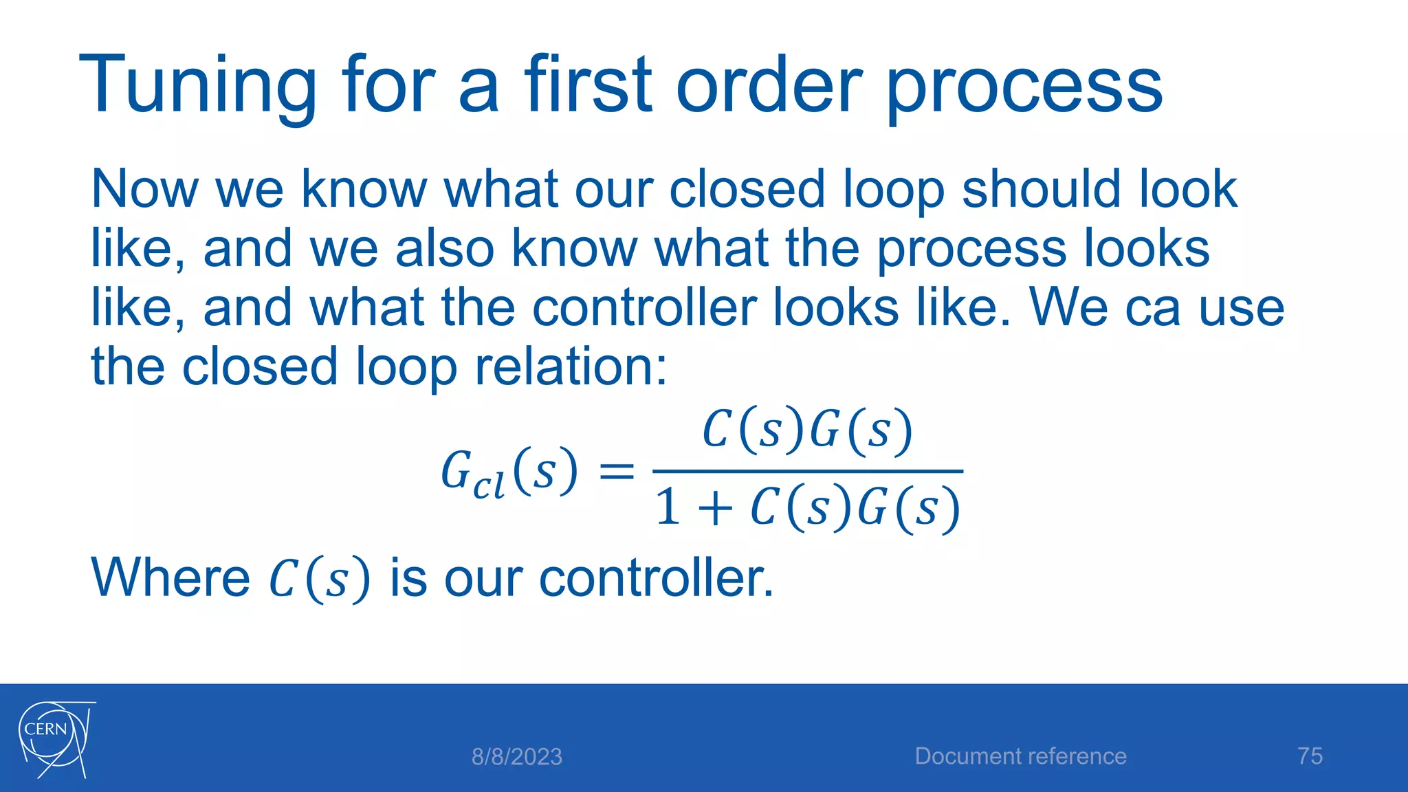
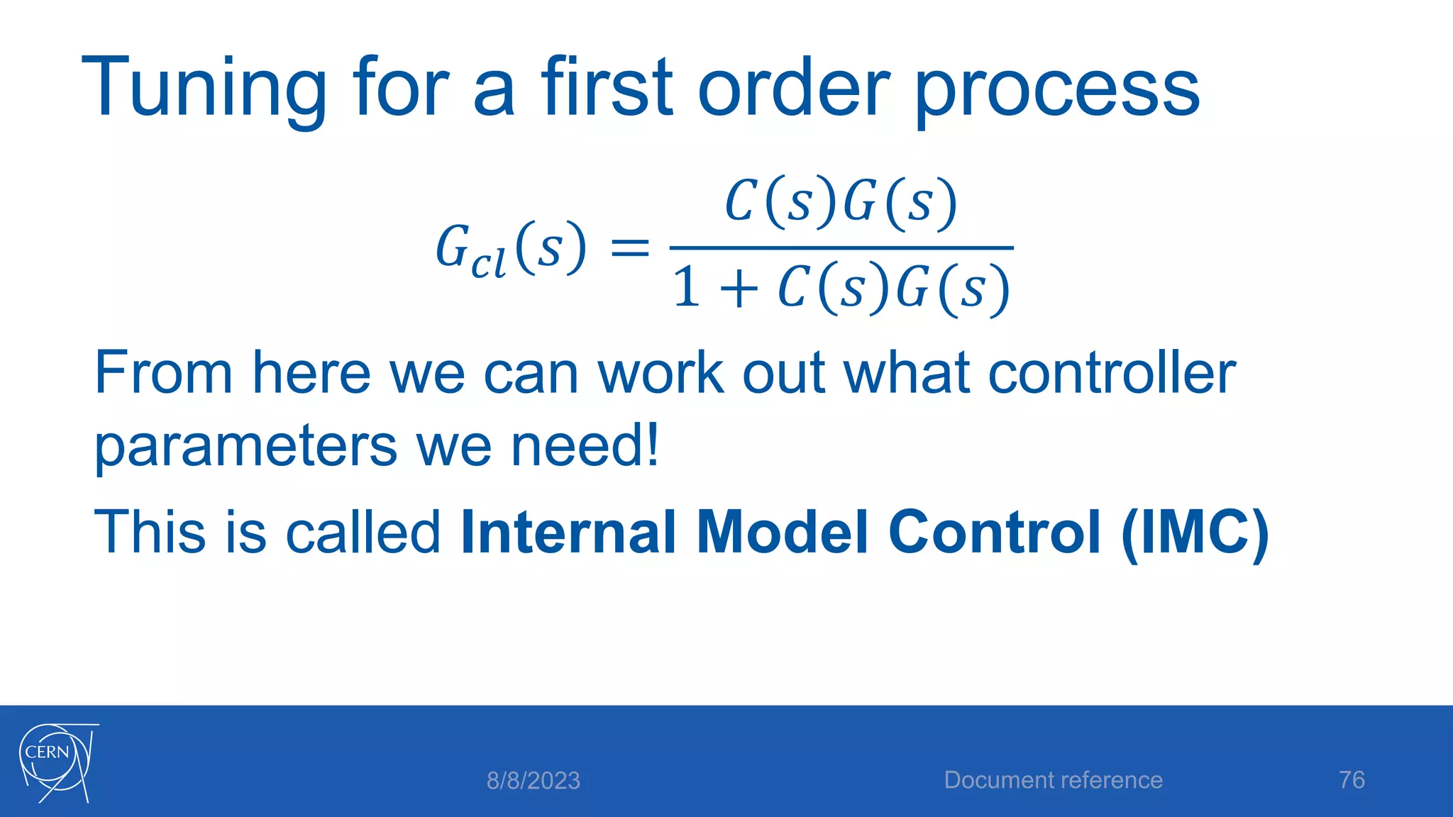
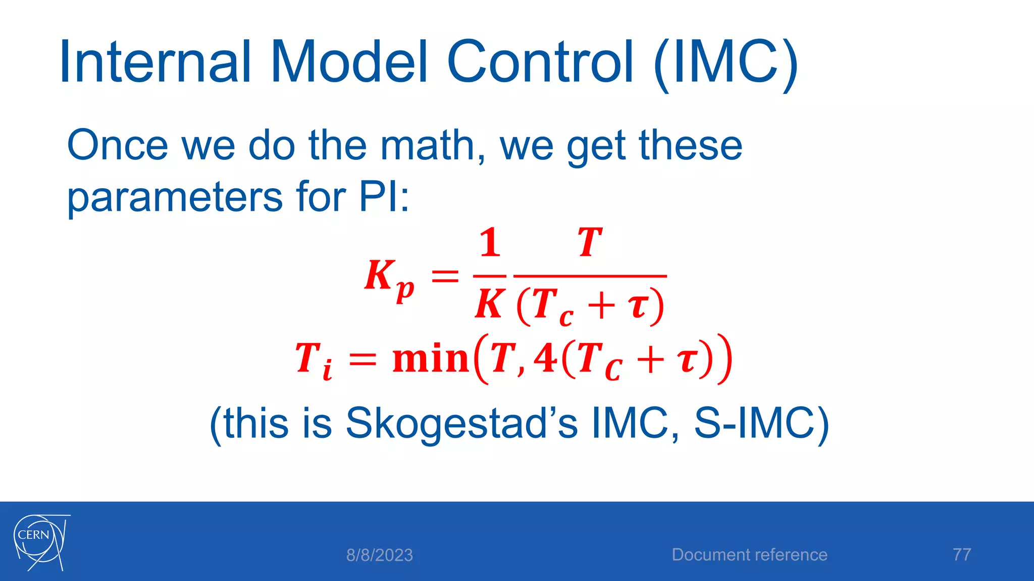
- The full PID control equation incorporating proportional, integral and derivative terms with their corresponding parameters - proportional gain, integral time and derivative time.