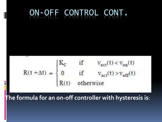
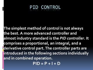
SlideShare a Scribd company logo
1 of 60
CONTROL
Closed loop control is an essential topic
for embedded systems, bringing
together actuators and sensors with the
control algorithm in software.
The central point of this chapter is to use motor
feedback via encoders for velocity control and
position control of motors.
We will exemplify this by a stepwise
introduction of PID (Proportional, Integral,
Derivative) control.
TYPES OF CONTROL
1- On-Off Control .
2- PID Control :
a. Proportional Controller .
b. Integral Controller .
c. Derivative Controller .
d. PID ParameterTuning .
3-Velocity Control and Position Control .
4- Multiple Motors – Driving Straight .
5-V-Omega Interface .
Feedback :
As we established before, we require feedback
on a motor’s current speed in
order to control it. Setting a certain PWM level
alone will not help, since the
motor’s speed also depends on its load
1- On-Off Control
The idea behind feedback control is very
simple. We have a desired speed, specified by
the user or the application program, and we
have the current actual speed, measured by
the shaft encoders. Measurements and actions
according to the measurements can be taken
very frequently, for example 100
times per second (Eye Bot) or up to 20,000
times per second.
On-Off Control cont.
ON-OFF CONTROL CONT.
The action taken depends on the controller model,
several of which are introduced in the following
sections. However, in principle the action always looks
similar like this:
• In case desired speed is higher than actual
speed:
Increase motor power by a certain degree.
• In case desired speed is lower than actual speed:
Decrease motor power by a certain degree.
In the simplest case, power to the motor is
either switched on (when thespeed is too low) or
switched off (when the speed is too high).This
control lawis represented by the formula below,
with:
On-Off Control cont.
R(t) motor output function over time t
vact(t) actual measured motor speed at time t
vdes(t) desired motor speed at time t
KC constant control value
KC if vact(t) < vdes(t)
R(t) =
0 otherwise
What has been defined here, is the concept of an
on-off controller, also known as “piecewise
constant controller” or “bang-bang controller”.
The motor input is set to constant value KC if the
measured velocity is too low, otherwise it is set to
zero. Note that this controller only works for a
positive value of vdes.The schematics diagram is
shown in Figure 5.1
On-Off Control
cont.
The behavior over time of an on-off ontroller is
shown in Figure 5.2. Assuming the motor is at
rest in the beginning, the actual speed is less
than the desired speed, so the control signal for
the motor is a constant voltage.This is kept until
at some stage the actual speed becomes larger
than the desired speed.
On-Off Control cont.
ON-OFF CONTROL CONT.
Now, the control signal is changed to zero. Over
some time, the actual speed will come down
again and once it falls below the desired speed,
the control signal will again be set to the same
constant voltage.This algorithm continues
indefinitely and can also accommodate changes
in the desired speed
ON-OFF CONTROL CONT.
Note that :
the motor control signal is not continuously
updated, but only at fixed time intervals (e.g.
every 10ms in Figure 5.2).This delay creates an
overshooting or undershooting of the actual
motor speed and thereby introduces hysteresis
HYSTERESIS
The on-off controller is the simplest possible
method of control. Many technical systems use
it, not limited to controlling a motor. Examples
are a refrigerator, heater, thermostat, etc. Most
of these technical systems use a hysteresis band,
which consists of two desired values, one for
switching on and one for switching off.This
prevents a too high switching frequency near the
desired value, in order to avoid excessive wear.
ON-OFF CONTROL CONT.
The formula for an on-off controller with hysteresis is:
ON-OFF CONTROL CONT.
Note that this definition is not a function in the
mathematical sense, because the new motor output
for an actual speed between the two band limit values
is equal to the previous motor value.This means it can
be equal to KC or zero in this case, depending on its
history. Figure 5.3 shows the hysteresis curve and the
corresponding control signal.
All technical systems have some delay and therefore
exhibit some inherent hysteresis, even if it is not
explicitly built-in
ON-OFF CONTROL CONT.
From theory to practice :
Once we understand the theory, we would like to
put this knowledge into practice and implement
an on-off controller in software.We will proceed
step by step:
1. We need a subroutine for calculating the motor
signal as defined in the formula in Figure 5.1. This
subroutine has to:
a. Read encoder data (input)
b. Compute new output value R(t)
c. Set motor speed (output)
2.This subroutine has to be called periodically (for
example every 1/100s). Since motor control is a
“low-level” task we would like this to run in the
background and not interfere with any user
program.
PID CONTROL
The simplest method of control is not always
the best. A more advanced controller and
almost industry standard is the PID controller. It
comprises a proportional, an integral, and a
derivative control part.The controller parts are
introduced in the following sections individually
and in combined operation.
PID = P + I + D
2.1 PROPORTIONAL CONTROLLER
For many control applications, the abrupt
change between a fixed motor control value and
zero does not result in a smooth control
behavior. We can improve this by using a linear
or proportional term instead.The formula for
the proportional controller (P controller) is:
R(t) = KP · (vdes(t) – vact(t))
2.1 PROPORTIONAL
CONTROLLER CONT.
The difference between the desired and actual speed is
called the “error function”. Figure 5.7 shows the
schematics for the P controller, which differs only
slightly from the on-off controller. Figure 5.8 shows
measurements of characteristic motor speeds over
time.Varying the “controller gain” KP will change the
controller behavior. The higher the KP chosen, the
faster the controller responds; however, a too high
value will lead to an undesirable oscillating system.
2.1 PROPORTIONAL
CONTROLLER CONT.
Therefore it is important to choose a value for KP that
guarantees a fast response but does not lead the control
system to overshoot too much or even oscillate
2.1 PROPORTIONAL
CONTROLLER CONT.
Steady state error : Note that the P controller’s
equilibrium state is not at the desired velocity. If the
desired speed is reached exactly, the motor output is
reduced to zero, as defined in the P controller formula
shown above.Therefore, each P controller will keep a
certain “steady-state error” from the desired velocity,
depending on the controller gain KP. As can be seen in
Figure 5.8, the higher the gain KP, the lower the
steady-state error. However, the system starts to
oscillate if the
selected gain is too high.
2.2 INTEGRAL CONTROLLER
Unlike the P controller, the I controller (integral
controller) is rarely used alone, but mostly in
combination with the P or PD controller. The idea for
the I controller is to reduce the steady-state error of the
P controller. With an additional integral term, this
steady-state error can be reduced to zero, as seen in the
measurements in Figure 5.9.The equilibrium state is
reached somewhat later than with a pure P controller,
but the steady-state error has been eliminated.
2.2 INTEGRAL CONTROLLER CONT.
When using e(t) as the error function, the
formula for the PI controller is:
R(t) = KP · [ e(t) + 1/TI · 0∫ t e(t)dt ]
We rewrite this formula by substituting
QI = KP/TI, so we receive independent
additive terms for P and I:
R(t) = KP · e(t) + QI · 0∫ t e(t)dt
2.2 INTEGRAL CONTROLLER CONT.
Naive approach :
The naive way of implementing the I controller part is to
transform the integration into a sum of a fixed number
(for example 10) of previous error values.
These 10 values would then have to be stored in an
array and added for every iteration.
2.2 INTEGRAL CONTROLLER CONT.
Proper PI implementation :The proper way of implementing a PI controller
starts with discretization, replacing the integral with a sum, using the
trapezoidal rule:
2.2 INTEGRAL CONTROLLER CONT.
Now we can get rid of the sum by using the
preceding output value Rn–1:
Rn – Rn–1 = KP · (en – en–1) + QI · tdelta · (en + en–1)/2
Therefore (substituting KI for QI · tdelta):
Rn = Rn–1 + KP · (en – en–1) + KI · (en + en–1)/2
2.3 DERIVATIVE CONTROLLER
Similar to the I controller, the D controller (derivative
controller) is rarely used by itself, but mostly in
combination with the P or PI controller.The idea for
adding a derivative term is to speed up the P controller’s
response to a change of input. Figure 5.10 shows the
measured differences of a step response between the P
and PD controller (top), and the PD and PID controller
(bottom).The PD controller reaches equilibrium faster
than the P controller, but still has a steady-state error.The
full PID controller combines the advantages of PI and PD.
It has a fast response and suffers no steady-state error.
2.3 DERIVATIVE CONTROLLER
CONT.
When using e(t) as the error function, the formula for
a combined PD controller
is:
R(t) = KP · [ e(t) +TD · de(t)/dt]
The formula for the full PID controller is:
R(t) = KP · [ e(t) + 1/TI · 0 ∫ t e(t)dt +TD · de(t)/dt ]
2.3 DERIVATIVE CONTROLLER
CONT.
Again, we rewrite this by substitutingTD andTI, so we
receive independent
additive terms for P, I, and D.This is important, in order
to experimentally
adjust the relative gains of the three terms.
R(t) = KP · e(t) + QI · 0 ∫ t e(t)dt + QD · de(t)/dt
2.4 PID PARAMETER TUNING
The tuning of the three PID parameters KP, KI, and KD is
an important issue.The following guidelines can be used
for experimentally finding suitable values (adapted after
[Williams 2006]):
1. Select a typical operating setting for the desired
speed, turn off integral and derivative parts, then
increase KP to maximum or until oscillation occurs.
2.4 PID PARAMETER
TUNING CONT.
2. If system oscillates, divide KP by 2.
3. Increase KD and observe behavior when increasing/decreasing the
desired speed by about 5%. Choose a value of KD which gives a damped
response.
4. Slowly increase KI until oscillation starts.Then divide KI by 2 or 3.
5. Check whether overall controller performance is satisfactorily under typical
system conditions
3. VELOCITY CONTROL AND
POSITION CONTROL
So far, we are able to control a single motor at a certain
speed, but we are not yet able to drive a motor at a
given speed for a number of revolutions and then come
to a stop at exactly the right motor position. The
former, maintaining a certain speed, is generally called
velocity control, while the latter, reaching a specified
position, is generally called position control.
3. VELOCITY CONTROL AND POSITION
CONTROL CONT.
Position control requires an additional controller on top
of the previously discussed velocity controller. The
position controller sets the desired velocities in all
driving phases, especially during the acceleration and
deceleration phases (starting and stopping).
3. VELOCITY CONTROL AND POSITION
CONTROL CONT.
Speed ramp: Let us assume a single motor is driving a
robot vehicle that is initially at rest and which we would
like to stop at a specified position. Figure 5.11
demonstrates the “speed ramp” for the starting phase,
constant speed phase, and stopping phase. When ignoring
friction, we only need to apply a certain force (here
constant) during the starting phase, which will translate
into an acceleration of the vehicle. The constant
acceleration will linearly increase the vehicle’s speed v
(integral of a) from 0 to the desired value vmax, while the
vehicle’s position s(integral of v) will increase quadratic
ally.
3. VELOCITY CONTROL AND POSITION
CONTROL CONT.
When the force (acceleration) stops, the vehicle’s
velocity will remain constant, assuming there is no
friction, and its position will increase linearly.
During the stopping phase (deceleration, braking), a
negative force (negative acceleration) is applied to the
vehicle. Its speed will be linearly reduced to
zero (or may even become negative – the vehicle now
driving backwards – if the negative acceleration is
applied for too long a time).The vehicle’s position
will increase slowly, following the square root function.
3. VELOCITY CONTROL AND POSITION
CONTROL CONT.
The tricky bit now is to control the amount of
acceleration in such a way that the vehicle:
a. Comes to rest (not moving slowly forward to
backward).
b. Comes to rest at exactly the specified position
(for example we want the vehicle to drive exactly 1
meter and stop within ±mm )
3. VELOCITY CONTROL AND POSITION
CONTROL CONT.
Figure 5.12 shows a way of achieving this by controlling
(continuously updating) the braking acceleration
applied.This control procedure has to take into account
not only the current speed as a feedback value, but also
the current position, since previous speed changes or
inaccuracies may have had already an effect on the
vehicle’s position.
4- MULTIPLE MOTORS – DRIVING
STRAIGHT
Unfortunately, this is still not the last of the motor
control problems. So far, we have only looked at a single
isolated motor with velocity control – and very briefly at
position control.The way that a robot vehicle is
constructed, however, shows us that a single motor is
not enough (see Figure 5.13)
4- MULTIPLE MOTORS – DRIVING
STRAIGHT CONT.
All these robot constructions require two motors, with
the functions of driving and steering either separated or
dependent on each other. In the design on the left or
the design on the right, the driving and steering
functions are separated. It is therefore very easy to
drive in a straight line (simply keep the steering fixed at
the angle representing “straight”) or drive in a circle
(keep the steering fixed at the appropriate angle).The
situation is quite different in the
4- MULTIPLE MOTORS – DRIVING
STRAIGHT CONT.
“differential steering” design shown in the middle of
Figure 5.13, which is a very popular design for small
mobile robots. Here, one has to constantly monitor and
update both motor speeds in order to drive straight.
Driving in a circle can be achieved by adding a constant
offset to one of the motors.Therefore, a
synchronization of the two motor speeds is required.
4- MULTIPLE MOTORS – DRIVING
STRAIGHT CONT.
There are a number of different approaches for driving
straight.The idea presented in the following is from
[Jones, Flynn, Seiger 1999]. Figure 5.14
shows the first try for a differential drive vehicle to drive
in a straight line.There are two separate control loops
for the left and the right motor, each
involving feedback control via a P controller. The
desired forward speed is supplied to both controllers .
Unfortunately, this design will not produce a nice
straight line of driving.
4- MULTIPLE MOTORS – DRIVING
STRAIGHT CONT.
Although each motor is controlled in itself, there is no
control of any slight speed discrepancies between the
two motors. Such a setup will most likely result in the
robot driving in a wriggly line, but not straight.
5- V-OMEGA INTERFACE
When programming a robot vehicle, we have to
abstract all the low-level motor control problems shown
in this chapter. Instead, we prefer to have a user-
friendly interface with specialized driving functions for a
vehicle that automatically takes care of all the feedback
control issues discussed.
5- V-OMEGA INTERFACE CONT.
We have implemented such a driving interface in the
RoBIOS operating system, called the “v-omega
interface”, because it allows us to specify a linear
and rotational speed of a robot vehicle. There are lower-
level functions for direct control of the motor speed, as
well as higher-level functions for driving a
complete trajectory in a straight line or a curve
(Program 5.8).
5- V-OMEGA INTERFACE CONT.
Dead reckoning The initialization of the vω interface
VWInit specifies the update rate of
motor commands, usually 1/100 of a second, but does
not activate PI control. The control routine,
VWStartControl, will start PI controllers for both driving
and steering as a background process with the PI
parameters supplied.The corresponding
timer interrupt routine contains all the program code for
controlling the two driving motors and updating the
internal variables for the vehicle’s
5- V-OMEGA INTERFACE CONT.
current position and orientation that can be read by
usingVWGetPosition. This method of determining a
vehicle’s position by continued addition of driving
vectors and maintaining its orientation by adding all
rotations is called “dead reckoning”. Function
VWStalled compares desired and actual motor speeds in
order to check whether the robot’s wheels have stalled,
possibly because it has collided with an obstacle.
Control

More Related Content

What's hot

Types of Controllers PID PD I PD
Types of Controllers PID PD I PDTypes of Controllers PID PD I PD
Types of Controllers PID PD I PDAnaseem Hanini
 
Speed control of dc motor using fuzzy pid controller-mid term progress report
Speed control of dc motor using fuzzy pid controller-mid term progress reportSpeed control of dc motor using fuzzy pid controller-mid term progress report
Speed control of dc motor using fuzzy pid controller-mid term progress reportBinod kafle
 
Fractional order-pid-controller design
Fractional order-pid-controller designFractional order-pid-controller design
Fractional order-pid-controller designRiyad Khazali
 
5. feedback control[1]
5. feedback control[1]5. feedback control[1]
5. feedback control[1]magy31
 
PID Controller and its design
PID Controller and its designPID Controller and its design
PID Controller and its designKonirDom1
 
Introduction to control system
Introduction to control systemIntroduction to control system
Introduction to control systemRosh54
 
Speed control of dc motor by fuzzy controller
Speed control of dc motor by fuzzy controllerSpeed control of dc motor by fuzzy controller
Speed control of dc motor by fuzzy controllerMurugappa Group
 
Level Control of Tank System Using PID Controller-A Review
Level Control of Tank System Using PID Controller-A ReviewLevel Control of Tank System Using PID Controller-A Review
Level Control of Tank System Using PID Controller-A ReviewIJSRD
 
Control Systems Basics
Control Systems BasicsControl Systems Basics
Control Systems BasicsJohn Todora
 
Pid controllers
Pid controllersPid controllers
Pid controllersHussain K
 
Fuzzy logic speed control of three phase
Fuzzy logic speed control of three phaseFuzzy logic speed control of three phase
Fuzzy logic speed control of three phaseaspafoto
 
Thompson tchobanian ni_li)
Thompson tchobanian ni_li)Thompson tchobanian ni_li)
Thompson tchobanian ni_li)trtrungviet
 
PID Control Basics
PID Control BasicsPID Control Basics
PID Control BasicsYokogawa1
 

What's hot (19)

Types of Controllers PID PD I PD
Types of Controllers PID PD I PDTypes of Controllers PID PD I PD
Types of Controllers PID PD I PD
 
Speed control of dc motor using fuzzy pid controller-mid term progress report
Speed control of dc motor using fuzzy pid controller-mid term progress reportSpeed control of dc motor using fuzzy pid controller-mid term progress report
Speed control of dc motor using fuzzy pid controller-mid term progress report
 
Fractional order-pid-controller design
Fractional order-pid-controller designFractional order-pid-controller design
Fractional order-pid-controller design
 
5. feedback control[1]
5. feedback control[1]5. feedback control[1]
5. feedback control[1]
 
Maintopik3
Maintopik3Maintopik3
Maintopik3
 
Pi controller ieee format
Pi controller ieee formatPi controller ieee format
Pi controller ieee format
 
PID Controller and its design
PID Controller and its designPID Controller and its design
PID Controller and its design
 
Introduction to control system
Introduction to control systemIntroduction to control system
Introduction to control system
 
Speed control of dc motor by fuzzy controller
Speed control of dc motor by fuzzy controllerSpeed control of dc motor by fuzzy controller
Speed control of dc motor by fuzzy controller
 
Pid controller
Pid controllerPid controller
Pid controller
 
Design of a discrete PID controller based on identification data for a simsca...
Design of a discrete PID controller based on identification data for a simsca...Design of a discrete PID controller based on identification data for a simsca...
Design of a discrete PID controller based on identification data for a simsca...
 
Level Control of Tank System Using PID Controller-A Review
Level Control of Tank System Using PID Controller-A ReviewLevel Control of Tank System Using PID Controller-A Review
Level Control of Tank System Using PID Controller-A Review
 
Control Systems Basics
Control Systems BasicsControl Systems Basics
Control Systems Basics
 
Pid controllers
Pid controllersPid controllers
Pid controllers
 
Fuzzy logic speed control of three phase
Fuzzy logic speed control of three phaseFuzzy logic speed control of three phase
Fuzzy logic speed control of three phase
 
Cs
CsCs
Cs
 
Thompson tchobanian ni_li)
Thompson tchobanian ni_li)Thompson tchobanian ni_li)
Thompson tchobanian ni_li)
 
PID Control Basics
PID Control BasicsPID Control Basics
PID Control Basics
 
Pid controller
Pid controllerPid controller
Pid controller
 

Viewers also liked (6)

Arithmatic &Logic Unit
Arithmatic &Logic UnitArithmatic &Logic Unit
Arithmatic &Logic Unit
 
Actuators
ActuatorsActuators
Actuators
 
Sensing
SensingSensing
Sensing
 
Introduction
IntroductionIntroduction
Introduction
 
Robotics Presentation
Robotics PresentationRobotics Presentation
Robotics Presentation
 
Robots presentation
Robots presentationRobots presentation
Robots presentation
 

Similar to Control

Servo Fundamentals
Servo FundamentalsServo Fundamentals
Servo Fundamentalspurnima saha
 
IRJET- Speed Control of Induction Motor using Hybrid PID Fuzzy Controller
IRJET- Speed Control of Induction Motor using Hybrid PID Fuzzy ControllerIRJET- Speed Control of Induction Motor using Hybrid PID Fuzzy Controller
IRJET- Speed Control of Induction Motor using Hybrid PID Fuzzy ControllerIRJET Journal
 
Control tutorials for matlab and simulink introduction pid controller desig...
Control tutorials for matlab and simulink   introduction pid controller desig...Control tutorials for matlab and simulink   introduction pid controller desig...
Control tutorials for matlab and simulink introduction pid controller desig...ssuser27c61e
 
PID controller in control systems
PID controller in control systemsPID controller in control systems
PID controller in control systemskhalaf Gaeid
 
Pid control by Adarsh singh
Pid control  by Adarsh singhPid control  by Adarsh singh
Pid control by Adarsh singhAdarsh Singh
 
Pid logix wp008--en-p
Pid logix wp008--en-pPid logix wp008--en-p
Pid logix wp008--en-pbenditasea
 
Real-time PID control of an inverted pendulum
Real-time PID control of an inverted pendulumReal-time PID control of an inverted pendulum
Real-time PID control of an inverted pendulumFrancesco Corucci
 
Introduction to control system 2
Introduction to control system 2Introduction to control system 2
Introduction to control system 2turna67
 
Controller ppt
Controller pptController ppt
Controller pptgourav0077
 
Meeting w12 chapter 4 part 2
Meeting w12   chapter 4 part 2Meeting w12   chapter 4 part 2
Meeting w12 chapter 4 part 2Hattori Sidek
 
Week 14 pid may 24 2016 pe 3032
Week  14 pid  may 24 2016 pe 3032Week  14 pid  may 24 2016 pe 3032
Week 14 pid may 24 2016 pe 3032Charlton Inao
 
Pid controllers
Pid controllersPid controllers
Pid controllersmilind1076
 

Similar to Control (20)

Servo Fundamentals
Servo FundamentalsServo Fundamentals
Servo Fundamentals
 
IRJET- Speed Control of Induction Motor using Hybrid PID Fuzzy Controller
IRJET- Speed Control of Induction Motor using Hybrid PID Fuzzy ControllerIRJET- Speed Control of Induction Motor using Hybrid PID Fuzzy Controller
IRJET- Speed Control of Induction Motor using Hybrid PID Fuzzy Controller
 
Chapter_8.ppt
Chapter_8.pptChapter_8.ppt
Chapter_8.ppt
 
Control tutorials for matlab and simulink introduction pid controller desig...
Control tutorials for matlab and simulink   introduction pid controller desig...Control tutorials for matlab and simulink   introduction pid controller desig...
Control tutorials for matlab and simulink introduction pid controller desig...
 
1578385.ppt
1578385.ppt1578385.ppt
1578385.ppt
 
PID controller in control systems
PID controller in control systemsPID controller in control systems
PID controller in control systems
 
PID controller
PID controllerPID controller
PID controller
 
Pid control by Adarsh singh
Pid control  by Adarsh singhPid control  by Adarsh singh
Pid control by Adarsh singh
 
Pid logix wp008--en-p
Pid logix wp008--en-pPid logix wp008--en-p
Pid logix wp008--en-p
 
Basicontrol
BasicontrolBasicontrol
Basicontrol
 
Real-time PID control of an inverted pendulum
Real-time PID control of an inverted pendulumReal-time PID control of an inverted pendulum
Real-time PID control of an inverted pendulum
 
4470838.ppt
4470838.ppt4470838.ppt
4470838.ppt
 
Introduction to control system 2
Introduction to control system 2Introduction to control system 2
Introduction to control system 2
 
Controller ppt
Controller pptController ppt
Controller ppt
 
Maintopik3
Maintopik3Maintopik3
Maintopik3
 
Meeting w12 chapter 4 part 2
Meeting w12   chapter 4 part 2Meeting w12   chapter 4 part 2
Meeting w12 chapter 4 part 2
 
PID Control
PID ControlPID Control
PID Control
 
Time Response
Time ResponseTime Response
Time Response
 
Week 14 pid may 24 2016 pe 3032
Week  14 pid  may 24 2016 pe 3032Week  14 pid  may 24 2016 pe 3032
Week 14 pid may 24 2016 pe 3032
 
Pid controllers
Pid controllersPid controllers
Pid controllers
 

Recently uploaded

Disha NEET Physics Guide for classes 11 and 12.pdf
Disha NEET Physics Guide for classes 11 and 12.pdfDisha NEET Physics Guide for classes 11 and 12.pdf
Disha NEET Physics Guide for classes 11 and 12.pdfchloefrazer622
 
Student login on Anyboli platform.helpin
Student login on Anyboli platform.helpinStudent login on Anyboli platform.helpin
Student login on Anyboli platform.helpinRaunakKeshri1
 
Nutritional Needs Presentation - HLTH 104
Nutritional Needs Presentation - HLTH 104Nutritional Needs Presentation - HLTH 104
Nutritional Needs Presentation - HLTH 104misteraugie
 
A Critique of the Proposed National Education Policy Reform
A Critique of the Proposed National Education Policy ReformA Critique of the Proposed National Education Policy Reform
A Critique of the Proposed National Education Policy ReformChameera Dedduwage
 
social pharmacy d-pharm 1st year by Pragati K. Mahajan
social pharmacy d-pharm 1st year by Pragati K. Mahajansocial pharmacy d-pharm 1st year by Pragati K. Mahajan
social pharmacy d-pharm 1st year by Pragati K. Mahajanpragatimahajan3
 
The byproduct of sericulture in different industries.pptx
The byproduct of sericulture in different industries.pptxThe byproduct of sericulture in different industries.pptx
The byproduct of sericulture in different industries.pptxShobhayan Kirtania
 
Grant Readiness 101 TechSoup and Remy Consulting
Grant Readiness 101 TechSoup and Remy ConsultingGrant Readiness 101 TechSoup and Remy Consulting
Grant Readiness 101 TechSoup and Remy ConsultingTechSoup
 
The basics of sentences session 2pptx copy.pptx
The basics of sentences session 2pptx copy.pptxThe basics of sentences session 2pptx copy.pptx
The basics of sentences session 2pptx copy.pptxheathfieldcps1
 
POINT- BIOCHEMISTRY SEM 2 ENZYMES UNIT 5.pptx
POINT- BIOCHEMISTRY SEM 2 ENZYMES UNIT 5.pptxPOINT- BIOCHEMISTRY SEM 2 ENZYMES UNIT 5.pptx
POINT- BIOCHEMISTRY SEM 2 ENZYMES UNIT 5.pptxSayali Powar
 
Kisan Call Centre - To harness potential of ICT in Agriculture by answer farm...
Kisan Call Centre - To harness potential of ICT in Agriculture by answer farm...Kisan Call Centre - To harness potential of ICT in Agriculture by answer farm...
Kisan Call Centre - To harness potential of ICT in Agriculture by answer farm...Krashi Coaching
 
Paris 2024 Olympic Geographies - an activity
Paris 2024 Olympic Geographies - an activityParis 2024 Olympic Geographies - an activity
Paris 2024 Olympic Geographies - an activityGeoBlogs
 
The Most Excellent Way | 1 Corinthians 13
The Most Excellent Way | 1 Corinthians 13The Most Excellent Way | 1 Corinthians 13
The Most Excellent Way | 1 Corinthians 13Steve Thomason
 
Ecosystem Interactions Class Discussion Presentation in Blue Green Lined Styl...
Ecosystem Interactions Class Discussion Presentation in Blue Green Lined Styl...Ecosystem Interactions Class Discussion Presentation in Blue Green Lined Styl...
Ecosystem Interactions Class Discussion Presentation in Blue Green Lined Styl...fonyou31
 
1029-Danh muc Sach Giao Khoa khoi 6.pdf
1029-Danh muc Sach Giao Khoa khoi  6.pdf1029-Danh muc Sach Giao Khoa khoi  6.pdf
1029-Danh muc Sach Giao Khoa khoi 6.pdfQucHHunhnh
 
Measures of Dispersion and Variability: Range, QD, AD and SD
Measures of Dispersion and Variability: Range, QD, AD and SDMeasures of Dispersion and Variability: Range, QD, AD and SD
Measures of Dispersion and Variability: Range, QD, AD and SDThiyagu K
 
Measures of Central Tendency: Mean, Median and Mode
Measures of Central Tendency: Mean, Median and ModeMeasures of Central Tendency: Mean, Median and Mode
Measures of Central Tendency: Mean, Median and ModeThiyagu K
 
Accessible design: Minimum effort, maximum impact
Accessible design: Minimum effort, maximum impactAccessible design: Minimum effort, maximum impact
Accessible design: Minimum effort, maximum impactdawncurless
 
Interactive Powerpoint_How to Master effective communication
Interactive Powerpoint_How to Master effective communicationInteractive Powerpoint_How to Master effective communication
Interactive Powerpoint_How to Master effective communicationnomboosow
 
Z Score,T Score, Percential Rank and Box Plot Graph
Z Score,T Score, Percential Rank and Box Plot GraphZ Score,T Score, Percential Rank and Box Plot Graph
Z Score,T Score, Percential Rank and Box Plot GraphThiyagu K
 

Recently uploaded (20)

Disha NEET Physics Guide for classes 11 and 12.pdf
Disha NEET Physics Guide for classes 11 and 12.pdfDisha NEET Physics Guide for classes 11 and 12.pdf
Disha NEET Physics Guide for classes 11 and 12.pdf
 
Student login on Anyboli platform.helpin
Student login on Anyboli platform.helpinStudent login on Anyboli platform.helpin
Student login on Anyboli platform.helpin
 
Nutritional Needs Presentation - HLTH 104
Nutritional Needs Presentation - HLTH 104Nutritional Needs Presentation - HLTH 104
Nutritional Needs Presentation - HLTH 104
 
A Critique of the Proposed National Education Policy Reform
A Critique of the Proposed National Education Policy ReformA Critique of the Proposed National Education Policy Reform
A Critique of the Proposed National Education Policy Reform
 
social pharmacy d-pharm 1st year by Pragati K. Mahajan
social pharmacy d-pharm 1st year by Pragati K. Mahajansocial pharmacy d-pharm 1st year by Pragati K. Mahajan
social pharmacy d-pharm 1st year by Pragati K. Mahajan
 
The byproduct of sericulture in different industries.pptx
The byproduct of sericulture in different industries.pptxThe byproduct of sericulture in different industries.pptx
The byproduct of sericulture in different industries.pptx
 
Grant Readiness 101 TechSoup and Remy Consulting
Grant Readiness 101 TechSoup and Remy ConsultingGrant Readiness 101 TechSoup and Remy Consulting
Grant Readiness 101 TechSoup and Remy Consulting
 
The basics of sentences session 2pptx copy.pptx
The basics of sentences session 2pptx copy.pptxThe basics of sentences session 2pptx copy.pptx
The basics of sentences session 2pptx copy.pptx
 
POINT- BIOCHEMISTRY SEM 2 ENZYMES UNIT 5.pptx
POINT- BIOCHEMISTRY SEM 2 ENZYMES UNIT 5.pptxPOINT- BIOCHEMISTRY SEM 2 ENZYMES UNIT 5.pptx
POINT- BIOCHEMISTRY SEM 2 ENZYMES UNIT 5.pptx
 
Kisan Call Centre - To harness potential of ICT in Agriculture by answer farm...
Kisan Call Centre - To harness potential of ICT in Agriculture by answer farm...Kisan Call Centre - To harness potential of ICT in Agriculture by answer farm...
Kisan Call Centre - To harness potential of ICT in Agriculture by answer farm...
 
Paris 2024 Olympic Geographies - an activity
Paris 2024 Olympic Geographies - an activityParis 2024 Olympic Geographies - an activity
Paris 2024 Olympic Geographies - an activity
 
The Most Excellent Way | 1 Corinthians 13
The Most Excellent Way | 1 Corinthians 13The Most Excellent Way | 1 Corinthians 13
The Most Excellent Way | 1 Corinthians 13
 
Ecosystem Interactions Class Discussion Presentation in Blue Green Lined Styl...
Ecosystem Interactions Class Discussion Presentation in Blue Green Lined Styl...Ecosystem Interactions Class Discussion Presentation in Blue Green Lined Styl...
Ecosystem Interactions Class Discussion Presentation in Blue Green Lined Styl...
 
1029-Danh muc Sach Giao Khoa khoi 6.pdf
1029-Danh muc Sach Giao Khoa khoi  6.pdf1029-Danh muc Sach Giao Khoa khoi  6.pdf
1029-Danh muc Sach Giao Khoa khoi 6.pdf
 
Measures of Dispersion and Variability: Range, QD, AD and SD
Measures of Dispersion and Variability: Range, QD, AD and SDMeasures of Dispersion and Variability: Range, QD, AD and SD
Measures of Dispersion and Variability: Range, QD, AD and SD
 
Measures of Central Tendency: Mean, Median and Mode
Measures of Central Tendency: Mean, Median and ModeMeasures of Central Tendency: Mean, Median and Mode
Measures of Central Tendency: Mean, Median and Mode
 
Accessible design: Minimum effort, maximum impact
Accessible design: Minimum effort, maximum impactAccessible design: Minimum effort, maximum impact
Accessible design: Minimum effort, maximum impact
 
Interactive Powerpoint_How to Master effective communication
Interactive Powerpoint_How to Master effective communicationInteractive Powerpoint_How to Master effective communication
Interactive Powerpoint_How to Master effective communication
 
Advance Mobile Application Development class 07
Advance Mobile Application Development class 07Advance Mobile Application Development class 07
Advance Mobile Application Development class 07
 
Z Score,T Score, Percential Rank and Box Plot Graph
Z Score,T Score, Percential Rank and Box Plot GraphZ Score,T Score, Percential Rank and Box Plot Graph
Z Score,T Score, Percential Rank and Box Plot Graph
 

Control

  • 1. CONTROL Closed loop control is an essential topic for embedded systems, bringing together actuators and sensors with the control algorithm in software.
  • 2. The central point of this chapter is to use motor feedback via encoders for velocity control and position control of motors. We will exemplify this by a stepwise introduction of PID (Proportional, Integral, Derivative) control.
  • 3. TYPES OF CONTROL 1- On-Off Control . 2- PID Control : a. Proportional Controller . b. Integral Controller . c. Derivative Controller . d. PID ParameterTuning . 3-Velocity Control and Position Control . 4- Multiple Motors – Driving Straight . 5-V-Omega Interface .
  • 4. Feedback : As we established before, we require feedback on a motor’s current speed in order to control it. Setting a certain PWM level alone will not help, since the motor’s speed also depends on its load 1- On-Off Control
  • 5. The idea behind feedback control is very simple. We have a desired speed, specified by the user or the application program, and we have the current actual speed, measured by the shaft encoders. Measurements and actions according to the measurements can be taken very frequently, for example 100 times per second (Eye Bot) or up to 20,000 times per second. On-Off Control cont.
  • 6. ON-OFF CONTROL CONT. The action taken depends on the controller model, several of which are introduced in the following sections. However, in principle the action always looks similar like this: • In case desired speed is higher than actual speed: Increase motor power by a certain degree. • In case desired speed is lower than actual speed: Decrease motor power by a certain degree.
  • 7. In the simplest case, power to the motor is either switched on (when thespeed is too low) or switched off (when the speed is too high).This control lawis represented by the formula below, with: On-Off Control cont.
  • 8. R(t) motor output function over time t vact(t) actual measured motor speed at time t vdes(t) desired motor speed at time t KC constant control value KC if vact(t) < vdes(t) R(t) = 0 otherwise
  • 9. What has been defined here, is the concept of an on-off controller, also known as “piecewise constant controller” or “bang-bang controller”. The motor input is set to constant value KC if the measured velocity is too low, otherwise it is set to zero. Note that this controller only works for a positive value of vdes.The schematics diagram is shown in Figure 5.1 On-Off Control cont.
  • 10.
  • 11. The behavior over time of an on-off ontroller is shown in Figure 5.2. Assuming the motor is at rest in the beginning, the actual speed is less than the desired speed, so the control signal for the motor is a constant voltage.This is kept until at some stage the actual speed becomes larger than the desired speed. On-Off Control cont.
  • 12.
  • 13. ON-OFF CONTROL CONT. Now, the control signal is changed to zero. Over some time, the actual speed will come down again and once it falls below the desired speed, the control signal will again be set to the same constant voltage.This algorithm continues indefinitely and can also accommodate changes in the desired speed
  • 14. ON-OFF CONTROL CONT. Note that : the motor control signal is not continuously updated, but only at fixed time intervals (e.g. every 10ms in Figure 5.2).This delay creates an overshooting or undershooting of the actual motor speed and thereby introduces hysteresis
  • 15. HYSTERESIS The on-off controller is the simplest possible method of control. Many technical systems use it, not limited to controlling a motor. Examples are a refrigerator, heater, thermostat, etc. Most of these technical systems use a hysteresis band, which consists of two desired values, one for switching on and one for switching off.This prevents a too high switching frequency near the desired value, in order to avoid excessive wear.
  • 16. ON-OFF CONTROL CONT. The formula for an on-off controller with hysteresis is:
  • 17. ON-OFF CONTROL CONT. Note that this definition is not a function in the mathematical sense, because the new motor output for an actual speed between the two band limit values is equal to the previous motor value.This means it can be equal to KC or zero in this case, depending on its history. Figure 5.3 shows the hysteresis curve and the corresponding control signal. All technical systems have some delay and therefore exhibit some inherent hysteresis, even if it is not explicitly built-in
  • 18.
  • 19. ON-OFF CONTROL CONT. From theory to practice : Once we understand the theory, we would like to put this knowledge into practice and implement an on-off controller in software.We will proceed step by step:
  • 20. 1. We need a subroutine for calculating the motor signal as defined in the formula in Figure 5.1. This subroutine has to: a. Read encoder data (input) b. Compute new output value R(t) c. Set motor speed (output) 2.This subroutine has to be called periodically (for example every 1/100s). Since motor control is a “low-level” task we would like this to run in the background and not interfere with any user program.
  • 21. PID CONTROL The simplest method of control is not always the best. A more advanced controller and almost industry standard is the PID controller. It comprises a proportional, an integral, and a derivative control part.The controller parts are introduced in the following sections individually and in combined operation. PID = P + I + D
  • 22. 2.1 PROPORTIONAL CONTROLLER For many control applications, the abrupt change between a fixed motor control value and zero does not result in a smooth control behavior. We can improve this by using a linear or proportional term instead.The formula for the proportional controller (P controller) is: R(t) = KP · (vdes(t) – vact(t))
  • 23. 2.1 PROPORTIONAL CONTROLLER CONT. The difference between the desired and actual speed is called the “error function”. Figure 5.7 shows the schematics for the P controller, which differs only slightly from the on-off controller. Figure 5.8 shows measurements of characteristic motor speeds over time.Varying the “controller gain” KP will change the controller behavior. The higher the KP chosen, the faster the controller responds; however, a too high value will lead to an undesirable oscillating system.
  • 24. 2.1 PROPORTIONAL CONTROLLER CONT. Therefore it is important to choose a value for KP that guarantees a fast response but does not lead the control system to overshoot too much or even oscillate
  • 25. 2.1 PROPORTIONAL CONTROLLER CONT. Steady state error : Note that the P controller’s equilibrium state is not at the desired velocity. If the desired speed is reached exactly, the motor output is reduced to zero, as defined in the P controller formula shown above.Therefore, each P controller will keep a certain “steady-state error” from the desired velocity, depending on the controller gain KP. As can be seen in Figure 5.8, the higher the gain KP, the lower the steady-state error. However, the system starts to oscillate if the selected gain is too high.
  • 26. 2.2 INTEGRAL CONTROLLER Unlike the P controller, the I controller (integral controller) is rarely used alone, but mostly in combination with the P or PD controller. The idea for the I controller is to reduce the steady-state error of the P controller. With an additional integral term, this steady-state error can be reduced to zero, as seen in the measurements in Figure 5.9.The equilibrium state is reached somewhat later than with a pure P controller, but the steady-state error has been eliminated.
  • 27.
  • 28. 2.2 INTEGRAL CONTROLLER CONT. When using e(t) as the error function, the formula for the PI controller is: R(t) = KP · [ e(t) + 1/TI · 0∫ t e(t)dt ] We rewrite this formula by substituting QI = KP/TI, so we receive independent additive terms for P and I: R(t) = KP · e(t) + QI · 0∫ t e(t)dt
  • 29. 2.2 INTEGRAL CONTROLLER CONT. Naive approach : The naive way of implementing the I controller part is to transform the integration into a sum of a fixed number (for example 10) of previous error values. These 10 values would then have to be stored in an array and added for every iteration.
  • 30.
  • 31. 2.2 INTEGRAL CONTROLLER CONT. Proper PI implementation :The proper way of implementing a PI controller starts with discretization, replacing the integral with a sum, using the trapezoidal rule:
  • 32. 2.2 INTEGRAL CONTROLLER CONT. Now we can get rid of the sum by using the preceding output value Rn–1: Rn – Rn–1 = KP · (en – en–1) + QI · tdelta · (en + en–1)/2 Therefore (substituting KI for QI · tdelta): Rn = Rn–1 + KP · (en – en–1) + KI · (en + en–1)/2
  • 33. 2.3 DERIVATIVE CONTROLLER Similar to the I controller, the D controller (derivative controller) is rarely used by itself, but mostly in combination with the P or PI controller.The idea for adding a derivative term is to speed up the P controller’s response to a change of input. Figure 5.10 shows the measured differences of a step response between the P and PD controller (top), and the PD and PID controller (bottom).The PD controller reaches equilibrium faster than the P controller, but still has a steady-state error.The full PID controller combines the advantages of PI and PD. It has a fast response and suffers no steady-state error.
  • 34.
  • 35.
  • 36. 2.3 DERIVATIVE CONTROLLER CONT. When using e(t) as the error function, the formula for a combined PD controller is: R(t) = KP · [ e(t) +TD · de(t)/dt] The formula for the full PID controller is: R(t) = KP · [ e(t) + 1/TI · 0 ∫ t e(t)dt +TD · de(t)/dt ]
  • 37. 2.3 DERIVATIVE CONTROLLER CONT. Again, we rewrite this by substitutingTD andTI, so we receive independent additive terms for P, I, and D.This is important, in order to experimentally adjust the relative gains of the three terms. R(t) = KP · e(t) + QI · 0 ∫ t e(t)dt + QD · de(t)/dt
  • 38. 2.4 PID PARAMETER TUNING The tuning of the three PID parameters KP, KI, and KD is an important issue.The following guidelines can be used for experimentally finding suitable values (adapted after [Williams 2006]): 1. Select a typical operating setting for the desired speed, turn off integral and derivative parts, then increase KP to maximum or until oscillation occurs.
  • 39. 2.4 PID PARAMETER TUNING CONT. 2. If system oscillates, divide KP by 2. 3. Increase KD and observe behavior when increasing/decreasing the desired speed by about 5%. Choose a value of KD which gives a damped response. 4. Slowly increase KI until oscillation starts.Then divide KI by 2 or 3. 5. Check whether overall controller performance is satisfactorily under typical system conditions
  • 40. 3. VELOCITY CONTROL AND POSITION CONTROL So far, we are able to control a single motor at a certain speed, but we are not yet able to drive a motor at a given speed for a number of revolutions and then come to a stop at exactly the right motor position. The former, maintaining a certain speed, is generally called velocity control, while the latter, reaching a specified position, is generally called position control.
  • 41. 3. VELOCITY CONTROL AND POSITION CONTROL CONT. Position control requires an additional controller on top of the previously discussed velocity controller. The position controller sets the desired velocities in all driving phases, especially during the acceleration and deceleration phases (starting and stopping).
  • 42. 3. VELOCITY CONTROL AND POSITION CONTROL CONT. Speed ramp: Let us assume a single motor is driving a robot vehicle that is initially at rest and which we would like to stop at a specified position. Figure 5.11 demonstrates the “speed ramp” for the starting phase, constant speed phase, and stopping phase. When ignoring friction, we only need to apply a certain force (here constant) during the starting phase, which will translate into an acceleration of the vehicle. The constant acceleration will linearly increase the vehicle’s speed v (integral of a) from 0 to the desired value vmax, while the vehicle’s position s(integral of v) will increase quadratic ally.
  • 43.
  • 44. 3. VELOCITY CONTROL AND POSITION CONTROL CONT. When the force (acceleration) stops, the vehicle’s velocity will remain constant, assuming there is no friction, and its position will increase linearly. During the stopping phase (deceleration, braking), a negative force (negative acceleration) is applied to the vehicle. Its speed will be linearly reduced to zero (or may even become negative – the vehicle now driving backwards – if the negative acceleration is applied for too long a time).The vehicle’s position will increase slowly, following the square root function.
  • 45. 3. VELOCITY CONTROL AND POSITION CONTROL CONT. The tricky bit now is to control the amount of acceleration in such a way that the vehicle: a. Comes to rest (not moving slowly forward to backward). b. Comes to rest at exactly the specified position (for example we want the vehicle to drive exactly 1 meter and stop within ±mm )
  • 46. 3. VELOCITY CONTROL AND POSITION CONTROL CONT. Figure 5.12 shows a way of achieving this by controlling (continuously updating) the braking acceleration applied.This control procedure has to take into account not only the current speed as a feedback value, but also the current position, since previous speed changes or inaccuracies may have had already an effect on the vehicle’s position.
  • 47.
  • 48. 4- MULTIPLE MOTORS – DRIVING STRAIGHT Unfortunately, this is still not the last of the motor control problems. So far, we have only looked at a single isolated motor with velocity control – and very briefly at position control.The way that a robot vehicle is constructed, however, shows us that a single motor is not enough (see Figure 5.13)
  • 49.
  • 50. 4- MULTIPLE MOTORS – DRIVING STRAIGHT CONT. All these robot constructions require two motors, with the functions of driving and steering either separated or dependent on each other. In the design on the left or the design on the right, the driving and steering functions are separated. It is therefore very easy to drive in a straight line (simply keep the steering fixed at the angle representing “straight”) or drive in a circle (keep the steering fixed at the appropriate angle).The situation is quite different in the
  • 51. 4- MULTIPLE MOTORS – DRIVING STRAIGHT CONT. “differential steering” design shown in the middle of Figure 5.13, which is a very popular design for small mobile robots. Here, one has to constantly monitor and update both motor speeds in order to drive straight. Driving in a circle can be achieved by adding a constant offset to one of the motors.Therefore, a synchronization of the two motor speeds is required.
  • 52.
  • 53. 4- MULTIPLE MOTORS – DRIVING STRAIGHT CONT. There are a number of different approaches for driving straight.The idea presented in the following is from [Jones, Flynn, Seiger 1999]. Figure 5.14 shows the first try for a differential drive vehicle to drive in a straight line.There are two separate control loops for the left and the right motor, each involving feedback control via a P controller. The desired forward speed is supplied to both controllers . Unfortunately, this design will not produce a nice straight line of driving.
  • 54. 4- MULTIPLE MOTORS – DRIVING STRAIGHT CONT. Although each motor is controlled in itself, there is no control of any slight speed discrepancies between the two motors. Such a setup will most likely result in the robot driving in a wriggly line, but not straight.
  • 55.
  • 56. 5- V-OMEGA INTERFACE When programming a robot vehicle, we have to abstract all the low-level motor control problems shown in this chapter. Instead, we prefer to have a user- friendly interface with specialized driving functions for a vehicle that automatically takes care of all the feedback control issues discussed.
  • 57. 5- V-OMEGA INTERFACE CONT. We have implemented such a driving interface in the RoBIOS operating system, called the “v-omega interface”, because it allows us to specify a linear and rotational speed of a robot vehicle. There are lower- level functions for direct control of the motor speed, as well as higher-level functions for driving a complete trajectory in a straight line or a curve (Program 5.8).
  • 58. 5- V-OMEGA INTERFACE CONT. Dead reckoning The initialization of the vω interface VWInit specifies the update rate of motor commands, usually 1/100 of a second, but does not activate PI control. The control routine, VWStartControl, will start PI controllers for both driving and steering as a background process with the PI parameters supplied.The corresponding timer interrupt routine contains all the program code for controlling the two driving motors and updating the internal variables for the vehicle’s
  • 59. 5- V-OMEGA INTERFACE CONT. current position and orientation that can be read by usingVWGetPosition. This method of determining a vehicle’s position by continued addition of driving vectors and maintaining its orientation by adding all rotations is called “dead reckoning”. Function VWStalled compares desired and actual motor speeds in order to check whether the robot’s wheels have stalled, possibly because it has collided with an obstacle.