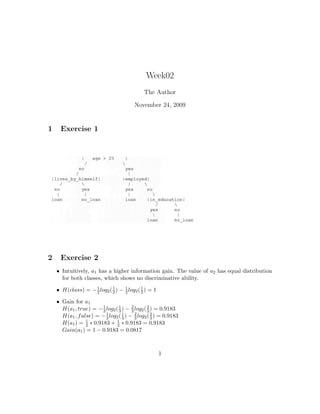
Week02
                                             The Author

                                        November 24, 2009


1    Exercise 1


2    Exercise 2
    • Intuitively, a1 has a higher information gain. The value of a2 has equal distribution
      for both classes, which shows no discriminative ability.

    • H(class) = − 1 log2 ( 1 ) − 1 log2 ( 2 ) = 1
                   2        2     2
                                           1


    • Gain for a1
      H(a1 , true) = − 1 log2 ( 1 ) − 2 log2 ( 3 ) = 0.9183
                       3        3      3
                                               2

      H(a1 , f alse) = − 3 log2 ( 3 ) − 3 log2 ( 2 ) = 0.9183
                         1        1      2
                                                 3
      H(a1 ) = 2 ∗ 0.9183 + 1 ∗ 0.9183 = 0.9183
                 1
                               2
      Gain(a1 ) = 1 − 0.9183 = 0.0817


                                                     1
studentID      score     class
                                      st1            9         yes
                                      st2            4         no
                                      st3            7         yes
                                      ...

                                  Table 1: Example of overfitting

    • Gain for a2
      H(a2 , true) = − 1 log2 ( 1 ) − 1 log2 ( 2 ) = 1
                       2        2      2
                                               1

      H(a2 , f alse) = − 2 log2 ( 2 ) − 2 log2 ( 1 ) = 1
                         1        1      1
                                                 2
                 1
      H(a2 ) = 2 ∗ 1 + 1 ∗ 1 = 1
                        2
      Gain(a2 ) = 1 − 1 = 0


3    Exercise 3
Assume we have following training example shown in Tab 3: For the attribute studentID,
it’s unique for each instance. In the training data, we can easily get the target class value
as long as know the studentID. However, this can not be generalized to unseen data, i.e.,
given a new studentID, we won’t be able to predict its class label.


4    Exercise 4
Example: if an attribute has n values, in an extreme case, we can have a data set of n
instances and each instance has a different value. Assume that we have a binary target,
then for each value of the attribute, the entropy of each value of the attribute is H(Sv ) =
−0 ∗ log2 0 − 1 ∗ log2 1 = 0
                                                               |Sv |
                          H(S, A) = H(S) −                           ∗ 0 = H(S)          (1)
                                                                |S|
                                                 v∈values(A)

since H(S, A) <= H(S), H(S) is the maximum gain we can have, so that the attribute in
this extreme case will always be selected by the information gain criterion. However, this
is not a good choice. (Consider the over-fitting problem discussed in exercise 3)


5    Exercise 5
    • Assign the most common value among examples for the missing value, i.e., “true” for
      attribute a1 at instance 2. In this case, we have
      gain(a1 ) = H(class) − H(class, a1 ) = H(class) − ( 3 H([2, 1]) + 1 H([1, 0]))
                                                          4             4


                                                    2
• A new value “missing” can be assigned to attribute a1 for instance 2. In this case,
  we have
  gain(a1 ) = H(class) − ( 1 H([1, 1]) + 1 H([1, 0]) + 1 H([1, 0]))
                           2             4             4


                                        3

Week02 answer

  • 1.
    Week02 The Author November 24, 2009 1 Exercise 1 2 Exercise 2 • Intuitively, a1 has a higher information gain. The value of a2 has equal distribution for both classes, which shows no discriminative ability. • H(class) = − 1 log2 ( 1 ) − 1 log2 ( 2 ) = 1 2 2 2 1 • Gain for a1 H(a1 , true) = − 1 log2 ( 1 ) − 2 log2 ( 3 ) = 0.9183 3 3 3 2 H(a1 , f alse) = − 3 log2 ( 3 ) − 3 log2 ( 2 ) = 0.9183 1 1 2 3 H(a1 ) = 2 ∗ 0.9183 + 1 ∗ 0.9183 = 0.9183 1 2 Gain(a1 ) = 1 − 0.9183 = 0.0817 1
  • 2.
    studentID score class st1 9 yes st2 4 no st3 7 yes ... Table 1: Example of overfitting • Gain for a2 H(a2 , true) = − 1 log2 ( 1 ) − 1 log2 ( 2 ) = 1 2 2 2 1 H(a2 , f alse) = − 2 log2 ( 2 ) − 2 log2 ( 1 ) = 1 1 1 1 2 1 H(a2 ) = 2 ∗ 1 + 1 ∗ 1 = 1 2 Gain(a2 ) = 1 − 1 = 0 3 Exercise 3 Assume we have following training example shown in Tab 3: For the attribute studentID, it’s unique for each instance. In the training data, we can easily get the target class value as long as know the studentID. However, this can not be generalized to unseen data, i.e., given a new studentID, we won’t be able to predict its class label. 4 Exercise 4 Example: if an attribute has n values, in an extreme case, we can have a data set of n instances and each instance has a different value. Assume that we have a binary target, then for each value of the attribute, the entropy of each value of the attribute is H(Sv ) = −0 ∗ log2 0 − 1 ∗ log2 1 = 0 |Sv | H(S, A) = H(S) − ∗ 0 = H(S) (1) |S| v∈values(A) since H(S, A) <= H(S), H(S) is the maximum gain we can have, so that the attribute in this extreme case will always be selected by the information gain criterion. However, this is not a good choice. (Consider the over-fitting problem discussed in exercise 3) 5 Exercise 5 • Assign the most common value among examples for the missing value, i.e., “true” for attribute a1 at instance 2. In this case, we have gain(a1 ) = H(class) − H(class, a1 ) = H(class) − ( 3 H([2, 1]) + 1 H([1, 0])) 4 4 2
  • 3.
    • A newvalue “missing” can be assigned to attribute a1 for instance 2. In this case, we have gain(a1 ) = H(class) − ( 1 H([1, 1]) + 1 H([1, 0]) + 1 H([1, 0])) 2 4 4 3