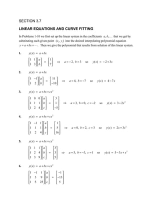
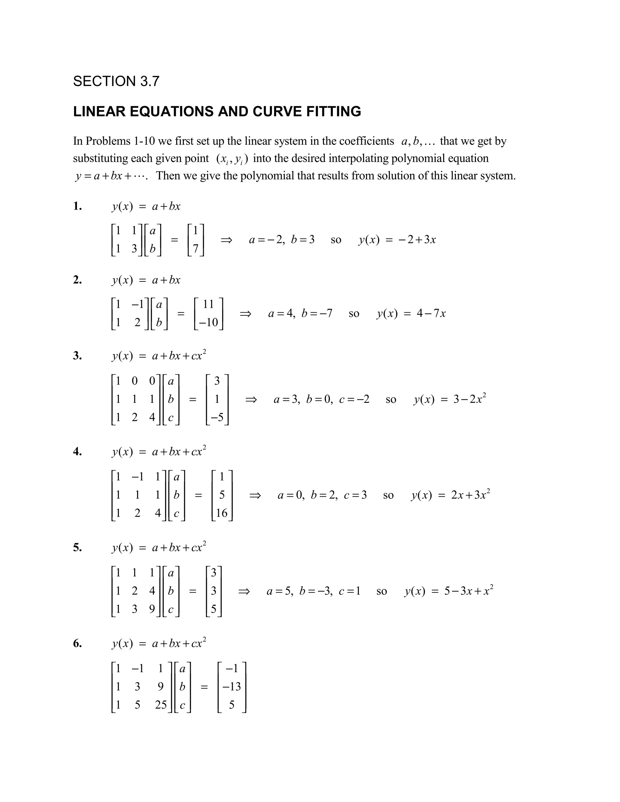
SECTION 3.7

LINEAR EQUATIONS AND CURVE FITTING

In Problems 1-10 we first set up the linear system in the coefficients a , b,  that we get by
substituting each given point ( xi , yi ) into the desired interpolating polynomial equation
 y = a + bx + . Then we give the polynomial that results from solution of this linear system.

1.      y ( x ) = a + bx

        1 1   a   1 
        1 3  b  = 7         ⇒   a = − 2, b = 3   so    y ( x) = − 2 + 3 x
                   

2.      y ( x ) = a + bx

        1 −1  a     11 
        1 2   b  =  −10         ⇒   a = 4, b = −7     so    y ( x) = 4 − 7 x
                        

3.      y ( x ) = a + bx + cx 2

        1 0 0   a    3
        1 1 1   b  =  1         ⇒    a = 3, b = 0, c = −2    so     y ( x) = 3 − 2 x 2
                      
        1 2 4   c 
                      −5 
                          

4.      y ( x ) = a + bx + cx 2

        1 −1 1   a   1
        1 1 1   b  =  5         ⇒     a = 0, b = 2, c = 3    so     y ( x) = 2 x + 3 x 2
                      
        1 2 4   c 
                     16 
                          

5.      y ( x ) = a + bx + cx 2

        1 1 1   a    3
        1 2 4   b  = 3          ⇒   a = 5, b = −3, c = 1    so    y ( x) = 5 − 3 x + x 2
                      
        1 3 9   c 
                     5 
                          

6.      y ( x ) = a + bx + cx 2

        1 −1 1   a   −1 
        1 3 9  b  =  −13
                        
        1 5 25   c 
                     5 
                            
⇒     a = − 10, b = −7, c = 2      so        y ( x) = − 10 − 7 x + 2 x 2

7.      y ( x ) = a + bx + cx 2 + dx 3

        1 −1  1 −1  a      1
        1 0         b 
               0 0          0
                            =  
        1 1   1 1  c       1
                            
        1 2   4 8  d        −4 
                           4
             ⇒ a = 0, b = , c = 1, d = −
                           3
                                         4
                                         3
                                                          so      y( x) =
                                                                            1
                                                                            3
                                                                              ( 4 x + 3x 2 − 4 x3 )
8.      y ( x ) = a + bx + cx 2 + dx 3

        1 −1     1 −1  a    3
        1 0           b 
                  0 0        5 
                             =  
        1 1      1 1  c     7 
                             
        1 2      4 8  d     3
             ⇒     a = 5, b = 3, c = 0, d = −1        so        y ( x) = 5 + 3x − x3

9.      y ( x ) = a + bx + cx 2 + dx 3

        1 −2 4 −8   a   −2 
        1 −1 1 −1  b    
                    =  2 
        1 1 1 1   c    10 
                        
        1 2 4 8   d     26 
             ⇒     a = 4, b = 3, c = 2, d = 1        so        y ( x) = 4 + 3 x + 2 x 2 + x 3

10.     y ( x ) = a + bx + cx 2 + dx 3

        1 −1     1 −1  a     17 
        1 1            b 
                  1 1          −5 
                              =  
        1 2      4 8  c      3
                              
        1 3      9 27   d     −2 
             ⇒     a = 17, b = −5, c = 3, d = −2           so       y ( x) = 17 − 5 x + 3 x 2 − 2 x 3

In Problems 11-14 we first set up the linear system in the coefficients A, B, C that we get by
substituting each given point ( xi , yi ) into the circle equation Ax + By + C = − x 2 − y 2 (see
Eq. (9) in the text). Then we give the circle that results from solution of this linear system.
11.     Ax + By + C = − x 2 − y 2

         −1 −1 1  A   −2 
         6 6 1  B  =  −72           ⇒      A = −6, B = −4, C = −12
                          
         7 5 1 C 
                      −74 
                              
        x 2 + y 2 − 6 x − 4 y − 12 = 0

        ( x − 3)2 + ( y − 2)2 = 25       center (3, 2) and radius 5

12.     Ax + By + C = − x 2 − y 2

         3 −4 1  A     −25 
         5 10 1  B  =  −125           ⇒     A = 6, B = −8, C = −75
                           
         −9 12 1 C 
                       −225
                               
        x 2 + y 2 + 6 x − 8 y − 75 = 0

        ( x + 3)2 + ( y − 4)2 = 100      center (–3, 4) and radius 10

13.     Ax + By + C = − x 2 − y 2

         1 0 1  A      −1 
         0 −5 1  B  =  −25           ⇒     A = 4, B = 4, C = −5
                           
         −5 −4 1 C 
                       −41
                               
        x2 + y 2 + 4 x + 4 y − 5 = 0

        ( x + 2)2 + ( y + 2)2 = 13       center (–3, –2) and radius     13

14.     Ax + By + C = − x 2 − y 2

         0 0 1  A     0 
        10 0 1  B  =  −100           ⇒     A = −10, B = −24, C = 0
                           
         −7 7 1 C 
                      −98 
                               
        x 2 + y 2 − 10 x − 24 y = 0

        ( x − 5)2 + ( y − 12)2 = 169     center (5, 12) and radius 13

In Problems 15-18 we first set up the linear system in the coefficients A, B, C that we get by
substituting each given point ( xi , yi ) into the central conic equation Ax 2 + Bxy + Cy 2 = 1 (see
Eq. (10) in the text). Then we give the equation that results from solution of this linear system.
15.   Ax 2 + Bxy + Cy 2 = 1

       0 0 25  A     1
       25 0 0   B  = 1             ⇒       A=
                                                      1       1
                                                         , B=− , C=
                                                                    1
                                                25      25    25
       25 25 25  C 
                     1
                         
      x 2 − xy + y 2 = 25


16.   Ax 2 + Bxy + Cy 2 = 1

       0   0   25   A    1
       25  0        B  = 1
                0                         ⇒     A=
                                                        1
                                                           , B=−
                                                                  7
                                                                     , C=
                                                                          1
                                                     25       100      25
      100 100 100  C 
                         1
                             
      4 x 2 − 7 xy + 4 y 2 = 100


17.   Ax 2 + Bxy + Cy 2 = 1

       0   0   1   A    1
       1   0   0   B  = 1              ⇒     A = 1, B = −
                                                                  199
                                                                      , C =1
                                                            100
      100 100 100  C 
                        1
                            
      100 x 2 − 199 xy + 100 y 2 = 100


18.   Ax 2 + Bxy + Cy 2 = 1

       0 0 16   A   1
       9 0 0   B  = 1              ⇒
                                                   1
                                                 A= , B =−
                                                            481
                                                                , C=
                                                                      1
                                             9       3600      16
       25 25 25 C 
                    1
                        
      400 x 2 − 481xy + 225 y 2 = 3600
                                                                               B
19.   We substitute each of the two given points into the equation y = A +       .
                                                                               x
      1 1 
       1   A = 5             ⇒   A = 3, B = 2 so y = 3 +
                                                                     2
      1    B   4
       2                                                       x
          
B C
20.     We substitute each of the three given points into the equation y = Ax +          + .
                                                                                        x x2
                  
        1    1 1
                    A  2
              1 1  
                       B =  20
        2                                                                                   8 16
                                           ⇒        A = 10, B = 8, C = −16 so y = 10 x +      −
             2 4                                                                       x x2
                    C    41
              1 1        
        4         
        
             4 16 
                   

In Problems 21 and 22 we fit the sphere equation ( x − h )2 + ( y − k )2 + ( z − l ) 2 = r 2 in the expanded
form Ax + By + Cz + D = − x 2 − y 2 − z 2 that is analogous to Eq. (9) in the text (for a circle).

21.      Ax + By + Cz + D = − x 2 − y 2 − z 2

         4 6 15         1  A   −277 
        13 5 7          1  B        
                            =  −243             ⇒     A = −2, B = −4, C = −6, D = −155
         5 14 6         1  C   −257 
                                    
         5 5 −9         1  D   −131
        x 2 + y 2 + z 2 − 2 x − 4 y − 6 z − 155 = 0

        ( x − 1)2 + ( y − 2)2 + ( z − 3)2 = 169       center (1, 2, 3) and radius 13

22.      Ax + By + Cz + D = − x 2 − y 2 − z 2

         11 17 17 1  A       −699 
         29           B
               1 15 1         −1067 
                             =                         ⇒     A = −10, B = 14, C = −18, D = −521
         13   −1 33 1  C     −1259 
                                   
         −19 −13 1 1  D      −531 
        x 2 + y 2 + z 2 − 10 x + 14 y − 18 z − 521 = 0

        ( x − 5) 2 + ( y + 7)2 + ( z − 9) 2 = 676     center (5, –7, 9) and radius 26

In Problems 23-26 we first take t = 0 in 1970 to fit a quadratic polynomial P(t ) = a + bt + ct 2 .
Then we write the quadratic polynomial Q(T ) = P(T − 1970) that expresses the predicted
population in terms of the actual calendar year T.
23.     P(t ) = a + bt + ct 2

        1 0   0  a      49.061
        1 10 100  b  =  49.137 
                               
        1 20 400   c 
                       50.809 
                                   
        P(t ) = 49.061 − 0.0722 t + 0.00798 t 2

        Q(T ) = 31160.9 − 31.5134 T + 0.00798 T 2

24.     P(t ) = a + bt + ct 2

        1 0   0  a     56.590 
        1 10 100  b  = 58.867 
                              
        1 20 400   c 
                       59.669 
                                  
        P(t ) = 56.590 + 0.30145 t − 0.007375 t 2

        Q(T ) = − 29158.9 + 29.3589 T − 0.007375 T 2


25.     P(t ) = a + bt + ct 2

        1 0   0  a      62.813 
        1 10 100  b  = 75.367 
                               
        1 20 400   c 
                       85.446 
                                   
        P(t ) = 62.813 + 1.37915 t − 0.012375 t 2

        Q(T ) = − 50680.3 + 50.1367 T − 0.012375 T 2


26.     P(t ) = a + bt + ct 2

        1 0   0  a     34.838
        1 10 100  b  =  43.171
                              
        1 20 400   c 
                       52.786 
                                  
        P(t ) = 34.838 + 0.7692 t + 0.00641t 2

        Q(T ) = 23396.1 − 24.4862 T + 0.00641T 2


In Problems 27-30 we first take t = 0 in 1960 to fit a cubic polynomial P(t ) = a + bt + ct 2 + dt 3 .
Then we write the cubic polynomial Q(T ) = P(T − 1960) that expresses the predicted population
in terms of the actual calendar year T.
27.   P(t ) = a + bt + ct 2 + dt 3

      1 0   0    0  a      44.678 
      1 10 100 1000   b           
                        =  49.061
      1 20 400 8000   c    49.137 
                                  
      1 30 900 27000   d  50.809 
      P(t ) = 44.678 + 0.850417 t − 0.05105 t 2 + 0.000983833 t 3

      Q(T ) = − 7.60554 × 10⁶ + 11539.4 T − 5.83599 T 2 + 0.000983833 T 3

28.   P(t ) = a + bt + ct 2 + dt 3

      1 0   0    0  a     51.619 
      1 10 100 1000   b          
                        = 56.590 
      1 20 400 8000   c   58.867 
                                 
      1 30 900 27000   d  59.669 
      P(t ) = 51.619 + 0.672433 t − 0.019565 t 2 + 0.000203167 t 3

      Q(T ) = − 1.60618 × 10⁶ + 2418.82 T − 1.21419 T 2 + 0.000203167 T 3

29.   P(t ) = a + bt + ct 2 + dt 3

      1 0   0    0  a      54.973 
      1 10 100 1000   b           
                        =  62.813
      1 20 400 8000   c   75.367 
                                  
      1 30 900 27000   d  85.446 
      P(t ) = 54.973 + 0.308667 t + 0.059515 t 2 − 0.00119817 t 3

      Q(T ) = 9.24972 ×10⁶ − 14041.6 T + 7.10474 T 2 − 0.00119817 T 3

30.   P(t ) = a + bt + ct 2 + dt 3

      1 0   0    0  a      28.053
      1 10 100 1000   b          
                        = 34.838 
      1 20 400 8000   c    43.171
                                 
      1 30 900 27000   d  52.786 
      P(t ) = 28.053 + 0.592233 t + 0.00907 t 2 − 0.0000443333 t 3

      Q(T ) = 367520 − 545.895 T + 0.26975 T 2 − 0.0000443333T 3
In Problems 31-34 we take t = 0 in 1950 to fit a quartic polynomial P(t ) = a + bt + ct 2 + dt 3 + et 4 .
Then we write the quartic polynomial Q(T ) = P(T − 1950) that expresses the predicted
population in terms of the actual calendar year T.

31.     P(t ) = a + bt + ct 2 + dt 3 + et 4 .

        1    0   0    0      0     a    39.478 
        1   10 100 1000            b 
                            10000        44.678 
                                                  
        1   20 400 8000 160000   c  =  49.061
                                               
        1   30 900 27000 810000   d     49.137 
        1
            40 1600 64000 2560000   e 
                                        50.809 
                                                   
        P(t ) = 39.478 + 0.209692 t + 0.0564163 t 2 − 0.00292992 t 3 + 0.0000391375 t 4

        Q(T ) = 5.87828 × 10⁸ − 1.19444 ×10⁶ T + 910.118 T 2 − 0.308202 T 3 + 0.0000391375 T 4

32.     P(t ) = a + bt + ct 2 + dt 3 + et 4 .

        1    0   0    0      0     a    44.461
        1   10 100 1000            b 
                            10000       51.619 
                                                 
        1   20 400 8000 160000   c  = 56.590 
                                              
        1   30 900 27000 810000   d    58.867 
        1
            40 1600 64000 2560000   e 
                                        59.669 
                                                  
        P(t ) = 44.461 + 0.7651t − 0.000489167 t 2 − 0.000516 t 3 + 7.19167 × 10⁻⁶ t 4

        Q(T ) = 1.07807 × 10⁸ − 219185 T + 167.096 T 2 − 0.056611T 3 + 7.19167 ×10⁻⁶ T 4

33.     P(t ) = a + bt + ct 2 + dt 3 + et 4 .

        1    0   0    0      0     a    47.197 
        1   10 100 1000            b 
                            10000        54.973 
                                                  
        1   20 400 8000 160000   c  =  62.813 
                                               
        1   30 900 27000 810000   d    75.367 
        1
            40 1600 64000 2560000   e 
                                        85.446 
                                                   
        P(t ) = 47.197 + 1.22537 t − 0.0771921t 2 + 0.00373475 t 3 − 0.0000493292 t 4

        Q(T ) = − 7.41239 × 10⁸ + 1.50598 × 10⁶ T − 1147.37 T 2 + 0.388502 T 3 − 0.0000493292 T 4
34.   P(t ) = a + bt + ct 2 + dt 3 + et 4 .

      1    0   0    0      0     a    20.190 
      1   10 100 1000            b 
                          10000        28.053
                                                
      1   20 400 8000 160000   c  = 34.838 
                                             
      1   30 900 27000 810000   d     43.171
      1
          40 1600 64000 2560000   e 
                                      52.786 
                                                 
      P(t ) = 20.190 + 1.00003 t − 0.031775 t 2 + 0.00116067 t 3 − 0.00001205 t 4

      Q(T ) = − 1.8296 ×10⁸ + 370762 T − 281.742 T 2 + 0.0951507 T 3 − 0.00001205 T 4

35.   Expansion of the determinant along the first row gives an equation of the form
       ay + bx 2 + cx + d = 0 that can be solved for y = Ax 2 + Bx + C. If the coordinates of any
      one of the three given points ( x1 , y1 ), ( x2 , y2 ), ( x3 , y3 ) are substituted in the first row, then
      the determinant has two identical rows and therefore vanishes.

36.   Expansion of the determinant along the first row gives

                  y       x2   x 1
                                       1 1 1    3 1 1  3 1 1 3 1 1
                  3       1    1 1
                                   = y 4 2 1−x 3 2 1+x 3 4 1− 3 4 2 =
                                              2

                  3       4    2 1
                                       9 3 1    7 3 1  7 9 1 7 9 3
                  7       9    3 1
                                              −2 y + 4 x 2 − 12 x + 14 = 0 .

      Hence y = 2 x 2 − 6 x + 7 is the parabola that interpolates the three given points.

37.   Expansion of the determinant along the first row gives an equation of the form
       a( x 2 + y 2 ) + bx + cy + d = 0, and we get the desired form of the equation of a circle upon
      division by a. If the coordinates of any one of the three given points ( x1 , y1 ), ( x2 , y2 ), and
       ( x3 , y3 ) are substituted in the first row, then the determinant has two identical rows and
      therefore vanishes.

38.   Expansion of the determinant along the first row gives

       x2 + y 2       x   y 1
         25           3 −4 1
                              =
        125           5 10 1
        225           −9 12 1
3 −4 1      25 −4 1      25 3 1 25 3 −4
               = ( x + y ) 5 10 1 − x 125 10 1 + y 125 5 1 − 125 5 10
                       2   2


                           −9 12 1    225 12 1     225 −9 1 225 −9 12

               = 200( x 2 + y 2 ) + 1200 x − 1600 y − 15000 = 0.

      Division by 200 and completion of squares gives ( x + 3)2 + ( y − 4)2 = 100, so the circle has
      center (–3, 4) and radius 10.

39.   Expansion of the determinant along the first row gives an equation of the form
      ax 2 + bxy + cy 2 + d = 0, which can be written in the central conic form
      Ax 2 + Bxy + Cy 2 = 1 upon division by –d. If the coordinates of any one of the three given
      points ( x1 , y1 ), ( x2 , y2 ), and ( x3 , y3 ) are substituted in the first row, then the determinant
      has two identical rows and therefore vanishes.

40.   Expansion of the determinant along the first row gives

       x2   y2 1
            xy
      0 0 16 1
                 =
      9 0 0 1
      25 25 25 1

                   0 16 1     0 16 1    0 0 1 0 0 16
               = x 0 0 1 − xy 9 0 1 + y 9 0 1 − 9 0 0
                   2


                   25 25 1    25 25 1   25 25 1 25 25 25

               = 400 x 2 − 481xy + 225 y 2 − 3600 = 0.

Sect3 7

  • 1.
    SECTION 3.7 LINEAR EQUATIONSAND CURVE FITTING In Problems 1-10 we first set up the linear system in the coefficients a , b, that we get by substituting each given point ( xi , yi ) into the desired interpolating polynomial equation y = a + bx + . Then we give the polynomial that results from solution of this linear system. 1. y ( x ) = a + bx 1 1   a  1  1 3  b  = 7  ⇒ a = − 2, b = 3 so y ( x) = − 2 + 3 x      2. y ( x ) = a + bx 1 −1  a   11  1 2   b  =  −10  ⇒ a = 4, b = −7 so y ( x) = 4 − 7 x      3. y ( x ) = a + bx + cx 2 1 0 0   a  3 1 1 1   b  =  1  ⇒ a = 3, b = 0, c = −2 so y ( x) = 3 − 2 x 2      1 2 4   c      −5    4. y ( x ) = a + bx + cx 2 1 −1 1   a  1 1 1 1   b  =  5  ⇒ a = 0, b = 2, c = 3 so y ( x) = 2 x + 3 x 2      1 2 4   c     16    5. y ( x ) = a + bx + cx 2 1 1 1   a  3 1 2 4   b  = 3 ⇒ a = 5, b = −3, c = 1 so y ( x) = 5 − 3 x + x 2      1 3 9   c     5    6. y ( x ) = a + bx + cx 2 1 −1 1   a   −1  1 3 9  b  =  −13      1 5 25   c      5   
  • 2.
    a = − 10, b = −7, c = 2 so y ( x) = − 10 − 7 x + 2 x 2 7. y ( x ) = a + bx + cx 2 + dx 3 1 −1 1 −1  a  1 1 0  b  0 0   0  =   1 1 1 1  c  1      1 2 4 8  d   −4  4 ⇒ a = 0, b = , c = 1, d = − 3 4 3 so y( x) = 1 3 ( 4 x + 3x 2 − 4 x3 ) 8. y ( x ) = a + bx + cx 2 + dx 3 1 −1 1 −1  a  3 1 0  b  0 0   5   =   1 1 1 1  c 7       1 2 4 8  d  3 ⇒ a = 5, b = 3, c = 0, d = −1 so y ( x) = 5 + 3x − x3 9. y ( x ) = a + bx + cx 2 + dx 3 1 −2 4 −8   a   −2  1 −1 1 −1  b       =  2  1 1 1 1   c  10       1 2 4 8   d   26  ⇒ a = 4, b = 3, c = 2, d = 1 so y ( x) = 4 + 3 x + 2 x 2 + x 3 10. y ( x ) = a + bx + cx 2 + dx 3 1 −1 1 −1  a  17  1 1  b  1 1    −5   =   1 2 4 8  c  3      1 3 9 27   d   −2  ⇒ a = 17, b = −5, c = 3, d = −2 so y ( x) = 17 − 5 x + 3 x 2 − 2 x 3 In Problems 11-14 we first set up the linear system in the coefficients A, B, C that we get by substituting each given point ( xi , yi ) into the circle equation Ax + By + C = − x 2 − y 2 (see Eq. (9) in the text). Then we give the circle that results from solution of this linear system.
  • 3.
    11. Ax + By + C = − x 2 − y 2  −1 −1 1  A   −2   6 6 1  B  =  −72  ⇒ A = −6, B = −4, C = −12       7 5 1 C      −74    x 2 + y 2 − 6 x − 4 y − 12 = 0 ( x − 3)2 + ( y − 2)2 = 25 center (3, 2) and radius 5 12. Ax + By + C = − x 2 − y 2  3 −4 1  A   −25   5 10 1  B  =  −125 ⇒ A = 6, B = −8, C = −75       −9 12 1 C      −225   x 2 + y 2 + 6 x − 8 y − 75 = 0 ( x + 3)2 + ( y − 4)2 = 100 center (–3, 4) and radius 10 13. Ax + By + C = − x 2 − y 2  1 0 1  A   −1   0 −5 1  B  =  −25  ⇒ A = 4, B = 4, C = −5       −5 −4 1 C      −41   x2 + y 2 + 4 x + 4 y − 5 = 0 ( x + 2)2 + ( y + 2)2 = 13 center (–3, –2) and radius 13 14. Ax + By + C = − x 2 − y 2  0 0 1  A   0  10 0 1  B  =  −100  ⇒ A = −10, B = −24, C = 0       −7 7 1 C      −98    x 2 + y 2 − 10 x − 24 y = 0 ( x − 5)2 + ( y − 12)2 = 169 center (5, 12) and radius 13 In Problems 15-18 we first set up the linear system in the coefficients A, B, C that we get by substituting each given point ( xi , yi ) into the central conic equation Ax 2 + Bxy + Cy 2 = 1 (see Eq. (10) in the text). Then we give the equation that results from solution of this linear system.
  • 4.
    15. Ax 2 + Bxy + Cy 2 = 1  0 0 25  A  1  25 0 0   B  = 1 ⇒ A= 1 1 , B=− , C= 1     25 25 25  25 25 25  C     1  x 2 − xy + y 2 = 25 16. Ax 2 + Bxy + Cy 2 = 1  0 0 25   A  1  25 0   B  = 1 0   ⇒ A= 1 , B=− 7 , C= 1   25 100 25 100 100 100  C     1  4 x 2 − 7 xy + 4 y 2 = 100 17. Ax 2 + Bxy + Cy 2 = 1  0 0 1   A 1  1 0 0   B  = 1 ⇒ A = 1, B = − 199 , C =1     100 100 100 100  C     1  100 x 2 − 199 xy + 100 y 2 = 100 18. Ax 2 + Bxy + Cy 2 = 1  0 0 16   A  1  9 0 0   B  = 1 ⇒ 1 A= , B =− 481 , C= 1     9 3600 16  25 25 25 C     1  400 x 2 − 481xy + 225 y 2 = 3600 B 19. We substitute each of the two given points into the equation y = A + . x 1 1   1   A = 5  ⇒ A = 3, B = 2 so y = 3 + 2 1  B 4  2     x  
  • 5.
    B C 20. We substitute each of the three given points into the equation y = Ax + + . x x2   1 1 1    A 2 1 1   B =  20 2 8 16 ⇒ A = 10, B = 8, C = −16 so y = 10 x + −  2 4     x x2  C   41 1 1     4    4 16   In Problems 21 and 22 we fit the sphere equation ( x − h )2 + ( y − k )2 + ( z − l ) 2 = r 2 in the expanded form Ax + By + Cz + D = − x 2 − y 2 − z 2 that is analogous to Eq. (9) in the text (for a circle). 21. Ax + By + Cz + D = − x 2 − y 2 − z 2  4 6 15 1  A   −277  13 5 7 1  B        =  −243  ⇒ A = −2, B = −4, C = −6, D = −155  5 14 6 1  C   −257        5 5 −9 1  D   −131 x 2 + y 2 + z 2 − 2 x − 4 y − 6 z − 155 = 0 ( x − 1)2 + ( y − 2)2 + ( z − 3)2 = 169 center (1, 2, 3) and radius 13 22. Ax + By + Cz + D = − x 2 − y 2 − z 2  11 17 17 1  A   −699   29  B 1 15 1    −1067   =   ⇒ A = −10, B = 14, C = −18, D = −521  13 −1 33 1  C   −1259        −19 −13 1 1  D   −531  x 2 + y 2 + z 2 − 10 x + 14 y − 18 z − 521 = 0 ( x − 5) 2 + ( y + 7)2 + ( z − 9) 2 = 676 center (5, –7, 9) and radius 26 In Problems 23-26 we first take t = 0 in 1970 to fit a quadratic polynomial P(t ) = a + bt + ct 2 . Then we write the quadratic polynomial Q(T ) = P(T − 1970) that expresses the predicted population in terms of the actual calendar year T.
  • 6.
    23. P(t ) = a + bt + ct 2 1 0 0  a   49.061 1 10 100  b  =  49.137       1 20 400   c     50.809    P(t ) = 49.061 − 0.0722 t + 0.00798 t 2 Q(T ) = 31160.9 − 31.5134 T + 0.00798 T 2 24. P(t ) = a + bt + ct 2 1 0 0  a  56.590  1 10 100  b  = 58.867       1 20 400   c     59.669    P(t ) = 56.590 + 0.30145 t − 0.007375 t 2 Q(T ) = − 29158.9 + 29.3589 T − 0.007375 T 2 25. P(t ) = a + bt + ct 2 1 0 0  a   62.813  1 10 100  b  = 75.367       1 20 400   c     85.446    P(t ) = 62.813 + 1.37915 t − 0.012375 t 2 Q(T ) = − 50680.3 + 50.1367 T − 0.012375 T 2 26. P(t ) = a + bt + ct 2 1 0 0  a  34.838 1 10 100  b  =  43.171      1 20 400   c     52.786    P(t ) = 34.838 + 0.7692 t + 0.00641t 2 Q(T ) = 23396.1 − 24.4862 T + 0.00641T 2 In Problems 27-30 we first take t = 0 in 1960 to fit a cubic polynomial P(t ) = a + bt + ct 2 + dt 3 . Then we write the cubic polynomial Q(T ) = P(T − 1960) that expresses the predicted population in terms of the actual calendar year T.
  • 7.
    27. P(t ) = a + bt + ct 2 + dt 3 1 0 0 0  a   44.678  1 10 100 1000   b        =  49.061 1 20 400 8000   c   49.137       1 30 900 27000   d  50.809  P(t ) = 44.678 + 0.850417 t − 0.05105 t 2 + 0.000983833 t 3 Q(T ) = − 7.60554 × 10⁶ + 11539.4 T − 5.83599 T 2 + 0.000983833 T 3 28. P(t ) = a + bt + ct 2 + dt 3 1 0 0 0  a  51.619  1 10 100 1000   b        = 56.590  1 20 400 8000   c  58.867       1 30 900 27000   d  59.669  P(t ) = 51.619 + 0.672433 t − 0.019565 t 2 + 0.000203167 t 3 Q(T ) = − 1.60618 × 10⁶ + 2418.82 T − 1.21419 T 2 + 0.000203167 T 3 29. P(t ) = a + bt + ct 2 + dt 3 1 0 0 0  a   54.973  1 10 100 1000   b        =  62.813 1 20 400 8000   c  75.367       1 30 900 27000   d  85.446  P(t ) = 54.973 + 0.308667 t + 0.059515 t 2 − 0.00119817 t 3 Q(T ) = 9.24972 ×10⁶ − 14041.6 T + 7.10474 T 2 − 0.00119817 T 3 30. P(t ) = a + bt + ct 2 + dt 3 1 0 0 0  a   28.053 1 10 100 1000   b        = 34.838  1 20 400 8000   c   43.171      1 30 900 27000   d  52.786  P(t ) = 28.053 + 0.592233 t + 0.00907 t 2 − 0.0000443333 t 3 Q(T ) = 367520 − 545.895 T + 0.26975 T 2 − 0.0000443333T 3
  • 8.
    In Problems 31-34we take t = 0 in 1950 to fit a quartic polynomial P(t ) = a + bt + ct 2 + dt 3 + et 4 . Then we write the quartic polynomial Q(T ) = P(T − 1950) that expresses the predicted population in terms of the actual calendar year T. 31. P(t ) = a + bt + ct 2 + dt 3 + et 4 . 1 0 0 0 0  a   39.478  1 10 100 1000  b  10000     44.678     1 20 400 8000 160000   c  =  49.061      1 30 900 27000 810000   d   49.137  1  40 1600 64000 2560000   e    50.809    P(t ) = 39.478 + 0.209692 t + 0.0564163 t 2 − 0.00292992 t 3 + 0.0000391375 t 4 Q(T ) = 5.87828 × 10⁸ − 1.19444 ×10⁶ T + 910.118 T 2 − 0.308202 T 3 + 0.0000391375 T 4 32. P(t ) = a + bt + ct 2 + dt 3 + et 4 . 1 0 0 0 0  a   44.461 1 10 100 1000  b  10000    51.619     1 20 400 8000 160000   c  = 56.590       1 30 900 27000 810000   d  58.867  1  40 1600 64000 2560000   e    59.669    P(t ) = 44.461 + 0.7651t − 0.000489167 t 2 − 0.000516 t 3 + 7.19167 × 10⁻⁶ t 4 Q(T ) = 1.07807 × 10⁸ − 219185 T + 167.096 T 2 − 0.056611T 3 + 7.19167 ×10⁻⁶ T 4 33. P(t ) = a + bt + ct 2 + dt 3 + et 4 . 1 0 0 0 0  a   47.197  1 10 100 1000  b  10000     54.973     1 20 400 8000 160000   c  =  62.813       1 30 900 27000 810000   d  75.367  1  40 1600 64000 2560000   e    85.446    P(t ) = 47.197 + 1.22537 t − 0.0771921t 2 + 0.00373475 t 3 − 0.0000493292 t 4 Q(T ) = − 7.41239 × 10⁸ + 1.50598 × 10⁶ T − 1147.37 T 2 + 0.388502 T 3 − 0.0000493292 T 4
  • 9.
    34. P(t ) = a + bt + ct 2 + dt 3 + et 4 . 1 0 0 0 0  a   20.190  1 10 100 1000  b  10000     28.053    1 20 400 8000 160000   c  = 34.838       1 30 900 27000 810000   d   43.171 1  40 1600 64000 2560000   e    52.786    P(t ) = 20.190 + 1.00003 t − 0.031775 t 2 + 0.00116067 t 3 − 0.00001205 t 4 Q(T ) = − 1.8296 ×10⁸ + 370762 T − 281.742 T 2 + 0.0951507 T 3 − 0.00001205 T 4 35. Expansion of the determinant along the first row gives an equation of the form ay + bx 2 + cx + d = 0 that can be solved for y = Ax 2 + Bx + C. If the coordinates of any one of the three given points ( x1 , y1 ), ( x2 , y2 ), ( x3 , y3 ) are substituted in the first row, then the determinant has two identical rows and therefore vanishes. 36. Expansion of the determinant along the first row gives y x2 x 1 1 1 1 3 1 1 3 1 1 3 1 1 3 1 1 1 = y 4 2 1−x 3 2 1+x 3 4 1− 3 4 2 = 2 3 4 2 1 9 3 1 7 3 1 7 9 1 7 9 3 7 9 3 1 −2 y + 4 x 2 − 12 x + 14 = 0 . Hence y = 2 x 2 − 6 x + 7 is the parabola that interpolates the three given points. 37. Expansion of the determinant along the first row gives an equation of the form a( x 2 + y 2 ) + bx + cy + d = 0, and we get the desired form of the equation of a circle upon division by a. If the coordinates of any one of the three given points ( x1 , y1 ), ( x2 , y2 ), and ( x3 , y3 ) are substituted in the first row, then the determinant has two identical rows and therefore vanishes. 38. Expansion of the determinant along the first row gives x2 + y 2 x y 1 25 3 −4 1 = 125 5 10 1 225 −9 12 1
  • 10.
    3 −4 1 25 −4 1 25 3 1 25 3 −4 = ( x + y ) 5 10 1 − x 125 10 1 + y 125 5 1 − 125 5 10 2 2 −9 12 1 225 12 1 225 −9 1 225 −9 12 = 200( x 2 + y 2 ) + 1200 x − 1600 y − 15000 = 0. Division by 200 and completion of squares gives ( x + 3)2 + ( y − 4)2 = 100, so the circle has center (–3, 4) and radius 10. 39. Expansion of the determinant along the first row gives an equation of the form ax 2 + bxy + cy 2 + d = 0, which can be written in the central conic form Ax 2 + Bxy + Cy 2 = 1 upon division by –d. If the coordinates of any one of the three given points ( x1 , y1 ), ( x2 , y2 ), and ( x3 , y3 ) are substituted in the first row, then the determinant has two identical rows and therefore vanishes. 40. Expansion of the determinant along the first row gives x2 y2 1 xy 0 0 16 1 = 9 0 0 1 25 25 25 1 0 16 1 0 16 1 0 0 1 0 0 16 = x 0 0 1 − xy 9 0 1 + y 9 0 1 − 9 0 0 2 25 25 1 25 25 1 25 25 1 25 25 25 = 400 x 2 − 481xy + 225 y 2 − 3600 = 0.