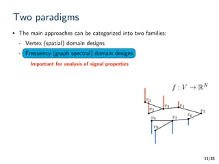
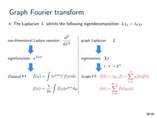
This document discusses graph signal processing and its applications. It begins by motivating the need to analyze structured data as graphs rather than as independent points. It then introduces basic concepts in graph signal processing such as representing data as graph signals on vertices, defining the graph Laplacian, and generalizing the Fourier transform to the graph spectral domain. The document outlines applications of graph signal processing tools like spectral filtering to domains such as social networks, transportation, and biomedicine.

1. Graph signal processing
Concepts, tools and applications
Xiaowen Dong
Department of Engineering Science

2. /35
Outline
2
• Motivation
• Graph signal processing (GSP): Basic concepts
• Spectral filtering: Basic tools of GSP
• Applications and perspectives

3. /35
Outline
2
• Motivation
• Graph signal processing (GSP): Basic concepts
• Spectral filtering: Basic tools of GSP
• Applications and perspectives

4. /35
Data are often structured
3
Electrical data Traffic data
Social network dataTemperature data

5. /35
Data are often structured
3
Electrical data Traffic data
Social network dataTemperature data
We need to take into account the structure behind the data

6. /35
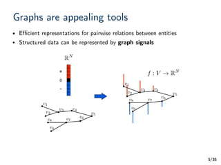
Graphs are appealing tools
4
l Efficient representations for pairwise relations between entities
The Königsberg Bridge Problem
[Leonhard Euler, 1736]

7. /35
Graphs are appealing tools
• Efficient representations for pairwise relations between entities
5
v1
v2
v3 v4
v5
v6v7v8
v9

8. /35
Graphs are appealing tools
• Efficient representations for pairwise relations between entities
5
l Structured data can be represented by graph signals
f : V ! RN
RN
+
0
-
v1
v2
v3 v4
v5
v6v7v8
v9
v1
v2
v3 v4
v5
v6v7v8
v9

9. /35
Graphs are appealing tools
• Efficient representations for pairwise relations between entities
5
l Structured data can be represented by graph signals
Takes into account both structure (edges) and data (values at vertices)
f : V ! RN
RN
+
0
-
v1
v2
v3 v4
v5
v6v7v8
v9
v1
v2
v3 v4
v5
v6v7v8
v9

10. /35
Graph signals are pervasive
6
• Vertices:
- 9000 grid cells in London
• Edges:
- Connecting cells that are
geographically close
• Signal:
- # Flickr users who have taken
photos in two and a half year

11. /35
Graph signals are pervasive
7
• Vertices:
- 1000 Twitter users
• Edges:
- Connecting users that have
following relationship
• Signal:
- # Apple-related hashtags they
have posted in six weeks

12. /35
Research challenges
8
How to generalize classical signal processing
tools on irregular domains such as graphs?
f : V ! RN
v1
v2
v3 v4
v5
v6v7v8
v9

13. /35
Graph signal processing
• Graph signals provide a nice compact format to encode structure within
data
• Generalization of classical signal processing tools can greatly benefit
analysis of such data
• Numerous applications: Transportation, biomedical,
social network analysis, etc.
• An increasingly rich literature
- classical signal processing
- algebraic and spectral graph theory
- computational harmonic analysis
9
f : V ! RN
v1
v2
v3 v4
v5
v6v7v8
v9

14. /35
Outline
10
• Motivation
• Graph signal processing (GSP): Basic concepts
• Spectral filtering: Basic tools of GSP
• Applications and perspectives

15. /35
Two paradigms
11
l The main approaches can be categorized into two families:
- Vertex (spatial) domain designs
- Frequency (graph spectral) domain designs
f : V ! RN
v1
v2
v3 v4
v5
v6v7v8
v9

16. /35
Two paradigms
11
l The main approaches can be categorized into two families:
- Vertex (spatial) domain designs
- Frequency (graph spectral) domain designs
Important for analysis of signal properties
f : V ! RN
v1
v2
v3 v4
v5
v6v7v8
v9

17. /35
Need for frequency
• Classical Fourier transform provides the frequency domain representation
of the signals
12
Source: http://www.physik.uni-kl.de
f : V ! RN
v1
v2
v3 v4
v5
v6v7v8
v9

18. /35
Need for frequency
• Classical Fourier transform provides the frequency domain representation
of the signals
12
Source: http://www.physik.uni-kl.de
A notion of frequency for graph signals:
We need the graph Laplacian matrix
f : V ! RN
v1
v2
v3 v4
v5
v6v7v8
v9

19. /35
Graph Laplacian
13
v1
v2
v3
v4 v5
v6
v7
v8
A
G = {V, E}
Weighted and undirected graph:

20. /35
Graph Laplacian
13
v1
v2
v3
v4 v5
v6
v7
v8
A
G = {V, E}
Weighted and undirected graph:
0
B
B
B
B
B
B
B
B
B
B
@
1 0 0 0 0 0 0 0
0 3 0 0 0 0 0 0
0 0 4 0 0 0 0 0
0 0 0 2 0 0 0 0
0 0 0 0 2 0 0 0
0 0 0 0 0 4 0 0
0 0 0 0 0 0 3 0
0 0 0 0 0 0 0 1
1
C
C
C
C
C
C
C
C
C
C
A
D
D = diag(degree(v1) ... degree(vN ))

21. L
/35
Graph Laplacian
13
v1
v2
v3
v4 v5
v6
v7
v8
L = D A
A
G = {V, E}
Weighted and undirected graph:
Equivalent to G!
0
B
B
B
B
B
B
B
B
B
B
@
1 0 0 0 0 0 0 0
0 3 0 0 0 0 0 0
0 0 4 0 0 0 0 0
0 0 0 2 0 0 0 0
0 0 0 0 2 0 0 0
0 0 0 0 0 4 0 0
0 0 0 0 0 0 3 0
0 0 0 0 0 0 0 1
1
C
C
C
C
C
C
C
C
C
C
A
D
D = diag(degree(v1) ... degree(vN ))

22. L
/35
Graph Laplacian
13
v1
v2
v3
v4 v5
v6
v7
v8
L = D A
A
G = {V, E}
Weighted and undirected graph:
Equivalent to G!
0
B
B
B
B
B
B
B
B
B
B
@
1 0 0 0 0 0 0 0
0 3 0 0 0 0 0 0
0 0 4 0 0 0 0 0
0 0 0 2 0 0 0 0
0 0 0 0 2 0 0 0
0 0 0 0 0 4 0 0
0 0 0 0 0 0 3 0
0 0 0 0 0 0 0 1
1
C
C
C
C
C
C
C
C
C
C
A
D
l Symmetric
l Off-diagonal entries non-positive
l Rows sum up to zero
D = diag(degree(v1) ... degree(vN ))

23. L
/35
Graph Laplacian
13
v1
v2
v3
v4 v5
v6
v7
v8
L = D A
A
G = {V, E}
Weighted and undirected graph:
Equivalent to G!
0
B
B
B
B
B
B
B
B
B
B
@
1 0 0 0 0 0 0 0
0 3 0 0 0 0 0 0
0 0 4 0 0 0 0 0
0 0 0 2 0 0 0 0
0 0 0 0 2 0 0 0
0 0 0 0 0 4 0 0
0 0 0 0 0 0 3 0
0 0 0 0 0 0 0 1
1
C
C
C
C
C
C
C
C
C
C
A
D
l Symmetric
l Off-diagonal entries non-positive
l Rows sum up to zero
D = diag(degree(v1) ... degree(vN ))
Why graph Laplacian?
- standard stencil approximation of the Laplace operator
- leads to a Fourier-like transform

24. /35
Graph Laplacian
14
f(1)
f(2)
f(3)
f(4)
f(5)
f(6)
f(7)
f(8)
Graph signal
L
f : V ! RN

25. /35
Graph Laplacian
14
f(1)
f(2)
f(3)
f(4)
f(5)
f(6)
f(7)
f(8)
A difference operator:
Graph signal
L
Lf =
NX
i,j=1
Aij (f(i) f(j))
f : V ! RN
f

26. /35
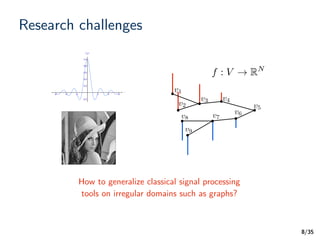
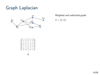
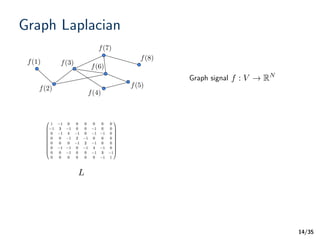
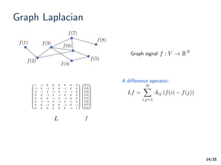
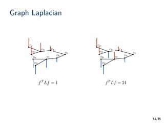
Graph Laplacian
14
f(1)
f(2)
f(3)
f(4)
f(5)
f(6)
f(7)
f(8)
A difference operator:
Graph signal
L
Laplacian quadratic form:
A measure of “smoothness” [Zhou04]
Lf =
NX
i,j=1
Aij (f(i) f(j))
fT
Lf =
1
2
NX
i,j=1
Aij (f(i) f(j))
2
f : V ! RN
f

27. /35
Graph Laplacian
15
v1
v2
v3 v4
v5
v6v7v8
v9
v1
v2
v3 v4
v5
v6v7v8
v9
fT
Lf = 1 fT
Lf = 21

28. /35
Graph Laplacian
• has a complete set of orthonormal eigenvectors:
16
L L = ⇤ T
2
6
4
0 0
...
0 N 1
3
7
5L
2
6
4
0 0
...
0 N 1
3
7
5· · ·0 N-1
2
6
4
0 0
...
0 N 1
3
7
5· · ·
0
N-1
⇤
T

29. /35
Graph Laplacian
• has a complete set of orthonormal eigenvectors:
16
L L = ⇤ T
2
6
4
0 0
...
0 N 1
3
7
5L
2
6
4
0 0
...
0 N 1
3
7
5· · ·0 N-1
2
6
4
0 0
...
0 N 1
3
7
5· · ·
0
N-1
l Eigenvalues are usually sorted increasingly: 0 = 0 < 1  . . .  N 1
⇤
T

30. /35
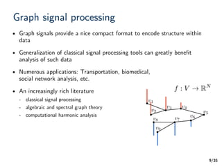
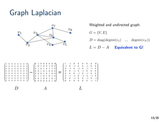
Graph Fourier transform
17
[Shuman13]0 501

31. /35
Graph Fourier transform
17
[Shuman13]0 501
Low frequency High frequency
T
50L 50 = 50
l Eigenvectors associated with smaller eigenvalues have values that vary less rapidly
along the edges
L = ⇤ T T
0 L 0 = 0 = 0

32. /35
Graph Fourier transform
17
[Shuman13]0 501
Low frequency High frequency
T
50L 50 = 50L = ⇤ T
fˆf(`) = h `, fi :
2
6
4
0 0
...
0 N 1
3
7
5· · ·0 N-1
T
Graph Fourier transform:
[Hammond11]
T
0 L 0 = 0 = 0

33. /35
Graph Fourier transform
17
[Shuman13]0 501
Low frequency High frequency
T
50L 50 = 50L = ⇤ T
Low frequency High frequency
fˆf(`) = h `, fi :
2
6
4
0 0
...
0 N 1
3
7
5· · ·0 N-1
T
Graph Fourier transform:
[Hammond11]
0 4
· · ·
· · ·1 2 3 N 1
T
0 L 0 = 0 = 0

34. /35
Graph Fourier transform
• The Laplacian admits the following eigendecomposition:
18
L ` = ` `L

35. /35
Graph Fourier transform
• The Laplacian admits the following eigendecomposition:
18
L ` = ` `L
one-dimensional Laplace operator:
d2
dx2
eigenfunctions: ej x
Classical FT:
f(x) =
1
2
Z
ˆf(⇥)ej x
d⇥
ˆf( ) =
Z
(ej x
)⇤
f(x)dx

36. /35
Graph Fourier transform
• The Laplacian admits the following eigendecomposition:
18
L ` = ` `L
one-dimensional Laplace operator:
d2
dx2
eigenfunctions: ej x
Classical FT:
f(x) =
1
2
Z
ˆf(⇥)ej x
d⇥
graph Laplacian:
eigenvectors: `
Graph FT: ˆf(⇥) = h , fi =
NX
i=1
⇤
(i)f(i)
f(i) =
N 1X
=0
ˆf(⇥) (i)
ˆf( ) =
Z
(ej x
)⇤
f(x)dx
L
f : V ! RN

37. /35
Graph Fourier transform
• The Laplacian admits the following eigendecomposition:
18
L ` = ` `L
one-dimensional Laplace operator:
d2
dx2
eigenfunctions: ej x
Classical FT:
f(x) =
1
2
Z
ˆf(⇥)ej x
d⇥
graph Laplacian:
eigenvectors: `
Graph FT: ˆf(⇥) = h , fi =
NX
i=1
⇤
(i)f(i)
f(i) =
N 1X
=0
ˆf(⇥) (i)
ˆf( ) =
Z
(ej x
)⇤
f(x)dx
L
f : V ! RN

38. /35
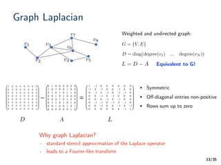
Two special cases
19
[Vandergheynst11]

39. /35
Two special cases
20
[Vandergheynst11]

40. /35
Outline
21
• Motivation
• Graph signal processing (GSP): Basic concepts
• Spectral filtering: Basic tools of GSP
• Applications and perspectives

41. /35
Classical frequency filtering
22
Classical FT: ˆf( ) =
Z
(ej x
)⇤
f(x)dx f(x) =
1
2
Z
ˆf(⇥)ej x
d⇥

42. /35
Classical frequency filtering
22
Classical FT: ˆf( ) =
Z
(ej x
)⇤
f(x)dx f(x) =
1
2
Z
ˆf(⇥)ej x
d⇥
Apply filter with transfer function to a signal
FT IFT
f
ˆg(·)
ˆf(!) ˆg(!) ˆf(!) f ⇤ g
ˆg(!)
f

43. /35
Classical frequency filtering
22
Classical FT: ˆf( ) =
Z
(ej x
)⇤
f(x)dx f(x) =
1
2
Z
ˆf(⇥)ej x
d⇥
Apply filter with transfer function to a signal
FT IFT
f
ˆg(·)
ˆf(!) ˆg(!) ˆf(!) f ⇤ g
ˆg(!)
f

44. /35
Graph spectral filtering
23
ˆf(`) = h `, fi =
NX
i=1
⇤
` (i)f(i) f(i) =
N 1X
`=0
ˆf(`) `(i)GFT:

45. /35
Graph spectral filtering
23
GFT IGFT
f
ˆf(`) = h `, fi =
NX
i=1
⇤
` (i)f(i) f(i) =
N 1X
`=0
ˆf(`) `(i)GFT:
ˆg( `)
ˆf(`) ˆg( `) ˆf(`) f(i) =
N 1X
`=0
ˆg( `) ˆf(`) `(i)
Apply filter with transfer function to a graph signal f : V ! Rn
ˆg(·)

46. /35
Graph spectral filtering
23
GFT IGFT
f
ˆf(`) = h `, fi =
NX
i=1
⇤
` (i)f(i) f(i) =
N 1X
`=0
ˆf(`) `(i)GFT:
ˆg( `)
ˆf(`) ˆg( `) ˆf(`) f(i) =
N 1X
`=0
ˆg( `) ˆf(`) `(i)
` ` `
Apply filter with transfer function to a graph signal f : V ! Rn
ˆg(·)

47. /35
Graph spectral filtering
23
ˆf(`) = h `, fi =
NX
i=1
⇤
` (i)f(i) f(i) =
N 1X
`=0
ˆf(`) `(i)GFT:
ˆg(⇤) =
2
6
4
ˆg( 0) 0
...
0 ˆg( N 1)
3
7
5
GFT IGFT
f T
f ˆg(⇤) T
f ˆg(⇤) T
f
ˆg(⇤)
Apply filter with transfer function to a graph signal f : V ! Rn
ˆg(·)

48. /35
Graph Laplacian revisited
24
ˆf(`) = h `, fi =
NX
i=1
⇤
` (i)f(i) f(i) =
N 1X
`=0
ˆf(`) `(i)GFT:

49. /35
Graph Laplacian revisited
24
The Laplacian is a difference operator:
GFT IGFT
f ⇤ T
f
ˆf(`) = h `, fi =
NX
i=1
⇤
` (i)f(i) f(i) =
N 1X
`=0
ˆf(`) `(i)GFT:
T
f ⇤ T
f
The Laplacian operator filters the signal in the spectral domain by its eigenvalues!
2
6
4
0 0
...
0 N 1
3
7
5
ˆg(⇤) = ⇤
L Lf = ⇤ T
f

50. /35
Graph Laplacian revisited
24
The Laplacian is a difference operator:
GFT IGFT
f ⇤ T
f
ˆf(`) = h `, fi =
NX
i=1
⇤
` (i)f(i) f(i) =
N 1X
`=0
ˆf(`) `(i)GFT:
T
f ⇤ T
f
The Laplacian operator filters the signal in the spectral domain by its eigenvalues!
The Laplacian quadratic form: fT
Lf = ||L
1
2 f||2 = || ⇤
1
2 T
f||2
2
6
4
0 0
...
0 N 1
3
7
5
ˆg(⇤) = ⇤
L Lf = ⇤ T
f

51. /35
Graph transform/dictionary design
• Transforms and dictionaries can be designed through graph spectral
filtering: Functions of graph Laplacian!
25
GFT IGFT
f T
f ˆg(⇤) T
f ˆg(⇤) T
f
ˆg(⇤)
ˆg(L)

52. /35
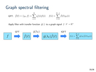
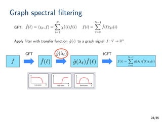
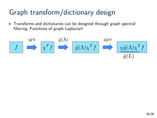
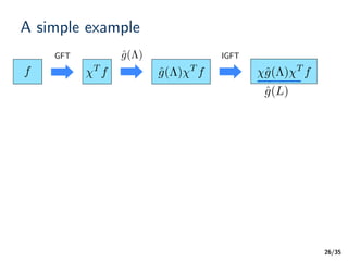
Graph transform/dictionary design
• Transforms and dictionaries can be designed through graph spectral
filtering: Functions of graph Laplacian!
25
GFT IGFT
f T
f ˆg(⇤) T
f ˆg(⇤) T
f
ˆg(⇤)
ˆg(L)
l Important properties can be achieved by properly defining , such
as localization of atoms
ˆg(L)
l Closely related to kernels and regularization on graphs [Smola03]

53. /35
A simple example
26
GFT IGFT
f T
f ˆg(⇤) T
f ˆg(⇤) T
f
ˆg(⇤)
ˆg(L)

54. /35
A simple example
26
GFT IGFT
f T
f ˆg(⇤) T
f ˆg(⇤) T
f
ˆg(⇤)
ˆg(L)
Problem: We observe a noisy graph signal and wish to recoverf = y0 + ⌘ y0
y⇤
= arg min
y
{||y f||2
2 + yT
Ly}

55. /35
A simple example
26
GFT IGFT
f T
f ˆg(⇤) T
f ˆg(⇤) T
f
ˆg(⇤)
ˆg(L)
Problem: We observe a noisy graph signal and wish to recoverf = y0 + ⌘ y0
y⇤
= arg min
y
{||y f||2
2 + yT
Ly}
Data fitting term
“Smoothness” assumption

56. /35
A simple example
26
GFT IGFT
f T
f ˆg(⇤) T
f ˆg(⇤) T
f
ˆg(⇤)
ˆg(L)
Problem: We observe a noisy graph signal and wish to recoverf = y0 + ⌘ y0
y⇤
= (I + L) 1
f
y⇤
= arg min
y
{||y f||2
2 + yT
Ly}
Data fitting term
“Smoothness” assumption
Laplacian (Tikhonov) regularization is equivalent to
low-pass filtering in the graph spectral domain!ˆg(L)

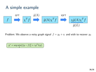
57. /35
Example designs
• Consider a noisy image as the observed noisy graph signal
• Consider a regular grid graph (weights inv. prop. to pixel value difference)
27
[Shuman13]

58. /35
Example designs
28
GFT IGFT
f T
f ˆg(⇤) T
f ˆg(⇤) T
f
ˆg(⇤)
ˆg(L)

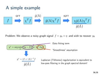
59. /35
Example designs
28
Low-pass filters:
Shifted and dilated band-pass filters: Spectral graph wavelets
Parametric polynomials:
Adapted kernels: Learn values of directly from data
GFT IGFT
f T
f ˆg(⇤) T
f ˆg(⇤) T
f
ˆg(⇤)
ˆg(L)
ˆg(L) = (I + L) 1
= (I + ⇤) 1 T
ˆgs(L) =
KX
k=0
↵skLk
= (
KX
k=0
↵sk⇤k
) T
ˆg(L) [Zhang12]
[Thanou14]
ˆg(sL) [Hammond11,
Shuman11, Dong13]
Window kernel: Windowed graph Fourier transform [Shuman12]

60. /35
Spectral graph wavelets
29
Fourier multiplier operator: scaled kernel ˆ⇤(s!)

61. /35
Spectral graph wavelets
29
Fourier multiplier operator: scaled kernel
dTs
g f(`) = g(s `) ˆf(`)
T
s
g
=
g(sL)
ˆ⇤(s!)

62. /35
Spectral graph wavelets
29
Fourier multiplier operator: scaled kernel
dTs
g f(`) = g(s `) ˆf(`)
(Ts
g f)(i) =
N 1X
=0
g(s ) ˆf(⇤)⇥ (i)
T
s
g
=
g(sL)
ˆ⇤(s!)

63. /35
Spectral graph wavelets
29
Fourier multiplier operator: scaled kernel
dTs
g f(`) = g(s `) ˆf(`)
(Ts
g f)(i) =
N 1X
=0
g(s ) ˆf(⇤)⇥ (i)
T
s
g
=
g(sL)
ˆ⇤(s!)

64. /35
Spectral graph wavelets
29
Fourier multiplier operator: scaled kernel
dTs
g f(`) = g(s `) ˆf(`)
(Ts
g f)(i) =
N 1X
=0
g(s ) ˆf(⇤)⇥ (i)
T
s
g
=
g(sL)
ˆ⇤(s!)

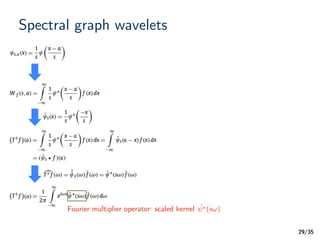
65. /35
Spectral graph wavelets
30
[Hammond11]

66. /35
Outline
31
• Motivation
• Graph signal processing (GSP): Basic concepts
• Spectral filtering: Basic tools of GSP
• Applications and perspectives

67. /35
Applications of GSP
• Signal processing and machine learning tasks
- Denoising [Graichen15, Liu16]
- Semi-supervised learning / Classification [Kipf16, Manessi17]
- Clustering [Tremblay14, Tremblay16]
- Dimensionality reduction [Rui16]
32

68. /35
Applications of GSP
• Signal processing and machine learning tasks
- Denoising [Graichen15, Liu16]
- Semi-supervised learning / Classification [Kipf16, Manessi17]
- Clustering [Tremblay14, Tremblay16]
- Dimensionality reduction [Rui16]
32
• Application domains
- Neuroimaging / Brain activity analysis [Huang16, Smith17, Ktena17]
- Social network analysis (e.g., community detection [Bruna17], recommendation
[Monti17], link prediction [Schlichtkrull17])
- Urban computing (e.g., mobility inference [Dong13])
- Computer graphics [Monti16, Yi16, Wang17, Simonovsky17]
- Geoscience and remote sensing [Bayram17]

69. /35
Future of GSP
• Mathematical models for graph signals
- global and local smoothness / regularity
- underlying physical processes
• Graph construction
- how to infer topologies given observed data?
• Fast implementation
- fast graph Fourier transform
- distributed processing
• Connection to / combination with other fields
- statistical machine learning
- deep learning (on graphs and manifolds)
• Applications
33

70. /35
References
• Three review papers:
34

71. /35
Resources
• Graph signal processing
- MATLAB toolbox: https://lts2.epfl.ch/gsp/
- Python toolbox: https://pygsp.readthedocs.io/en/stable/
• Spectral graph wavelet transform
- MATLAB toolbox: https://wiki.epfl.ch/sgwt
- Python toolbox: https://github.com/aweinstein/pysgwt
• Topology inference
- Tutorial: http://web.media.mit.edu/~xdong/presentation/GSPW_GraphLearning.pdf
• Geometric deep learning
- Workshops, tutorials, papers and code: http://geometricdeeplearning.com
35
contact: xiaowen.dong@eng.ox.ac.uk