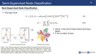
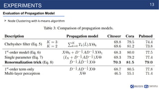
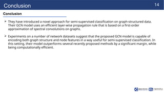
The document presents a novel approach for semi-supervised classification of nodes in graphs using a graph convolutional network (GCN) model that incorporates an efficient layer-wise propagation rule. This method improves classification accuracy and computational efficiency compared to state-of-the-art techniques. Experiments demonstrate the model's effectiveness in encoding graph structure and node features for classification tasks.


![[DL Hacks]Semi-Supervised Classification with Graph Convolutional Networks](https://cdn.slidesharecdn.com/ss_thumbnails/gcn1-181102025619-thumbnail.jpg?width=640&height=640&fit=bounds)


![[NS][Lab_Seminar_240710]Improving Graph Networks through Selection-based Conv...](https://cdn.slidesharecdn.com/ss_thumbnails/nslabseminar240710selgcn-240723105252-3f46ad9d-thumbnail.jpg?width=640&height=640&fit=bounds)


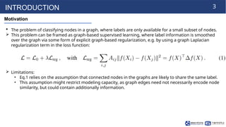
![241125_JW_labseminar[Simple and Deep Graph Convolutional Networks].pptx](https://cdn.slidesharecdn.com/ss_thumbnails/241125jwlabseminargcnii-241125095533-a294558a-thumbnail.jpg?width=640&height=640&fit=bounds)
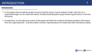
![250623_JW_labseminar[STRATEGIES FOR PRE-TRAINING GRAPH NEURAL NETWORKS].pptx](https://cdn.slidesharecdn.com/ss_thumbnails/250623jwlabseminarcontextpred-250627073644-0949d35d-thumbnail.jpg?width=640&height=640&fit=bounds)


![[NS][Lab_Seminar_260126]MIHC: Multi-View Interpretable Hypergraph Neural Netw...](https://cdn.slidesharecdn.com/ss_thumbnails/nslabseminar260126-260126110047-559006b2-thumbnail.jpg?width=640&height=640&fit=bounds)
![260119_SH_LabSeminar[ENGRAM]_최종2_최종3_4.pdf](https://cdn.slidesharecdn.com/ss_thumbnails/260119shlabseminarengram234-260120052642-29f38c8f-thumbnail.jpg?width=640&height=640&fit=bounds)


![[NS][Lab_Seminar_260119][DHGFormer: Dynamic Hierarchical Graph Transformer fo...](https://cdn.slidesharecdn.com/ss_thumbnails/nslabseminar260119-260120052625-9b28e6ed-thumbnail.jpg?width=640&height=640&fit=bounds)


![260105_JH_LabSeminar[A Plant-Wide Industrial Process Control Problem].pptx](https://cdn.slidesharecdn.com/ss_thumbnails/260105jhlabseminartep-260106063928-34e9f1f6-thumbnail.jpg?width=640&height=640&fit=bounds)


