W1_Lecture Notes nptel Distributed system

Lecture: 01
Introduction to Distributed
Systems
Rajiv Misra
Dept. of Computer Science & Engineering
Indian Institute of Technology Patna
rajivm@iitp.ac.in
N
P
T
E
L

Preface
• The explosive growth of DCS makes understanding imperative
yet difficult because of uncertainties introduced by
asynchrony, limited local knowledge, and partial failures.
• The nature solves it perfectly such as flock of birds( mobile
intelligent agents communicates to achieve common goal).
• The field of distributed computing provides theoretical
underpinning for design and analysis of many DS such as-
communication, coordination, synchronization and
uncertainty to lower bound techniques.
N
P
T
E
L

Course Contents
 Introduction to Distributed Systems
 Basic Algorithms in Message Passing System
 Leader Election in Rings
 Distributed Minimum Spanning Tree
 Models of Distributed Computation
 Causality & Logical Time
 Global State and Snapshot Recording
Algorithms
 Distributed Mutual Exclusion Algorithms
 Distributed Shared Memory
 Consensus and Agreement Algorithms
 Checkpointing & Rollback Recovery
Case Studies:
 Distributed Hash Table
 Peer to Peer Computing and
Overlay Graphs
 Google File System
 HDFS and Map Reduce
 Introduction to Spark
 Introduction to Sensor Networks
N
P
T
E
L

Books
Text Books:
• Distributed Computing: Principles, Algorithms, and Systems-
Ajay D. Kshemkalyani and Mukesh Singhal
• Distributed Computing: Fundamentals, Simulations and Advanced Topics-
Hagit Attiya and Jennifer Welch
Reference Book:
• Distributed Algorithms-
Nancy Lynch
N
P
T
E
L

Distributed System: Definition
• A distributed system is
• A collection of independent entities that cooperate to solve a
problem that cannot be individually solved.
• A collection of computers that do not share common
memory or a common physical clock, that communicate by
a messages passing over a communication network, and
where each computer has its own memory and runs its own
operating system.
• Typically the computers are semi-autonomous and are loosely coupled
while they cooperate to address a problem collectively.
N
P
T
E
L

Properties of Distributed Systems
• Heterogeneity
• Systems consist of heterogeneous hardware and software components
• Concurrency
• Multiple programs run together
• Shared data
• Data is accessed simultaneously by multiple entities
• No global clock
• Each component has a local notion of time
• Interdependencies
• Independent components depend on each other
N
P
T
E
L

Relation to Computer System Components
Figure 1.1: A typical distributed system
Communication
network
(WAN/ LAN)
P processor(s)
M memory bank(s)
P M
S/W
OS
P M
S/W
OS
P M
S/W
OS
Middleware
N
P
T
E
L

Relation to Computer System Components
• A DS connects autonomous processors by communication network
which cooperate to run application network.
• The software components that run on each of the computers use the
local operating system and network protocol stack for functioning.
• The distributed software is also termed as middleware.
• A distributed execution is the execution of processes across the
distributed system to collaboratively achieve a common goal. An
execution is also sometimes termed a computation or a run.
N
P
T
E
L

Layered Architecture
• The middleware(layered architecture) is the distributed software that drives the
distributed system, while providing transparency of heterogeneity at the platform
level.
Distributed application
Distributed software
(middleware libraries)
Network
protocol
stack
Operating
system
Application layer
Transport layer
Network layer
Data link layer
Figure 1.2: Layered Architecture of Distributed System
Application
Several standards as :
OMG (Object
Management Group )
CORBA (Common Object
Request Broker
Architecture)
RPC (Remote Procedure
Call)
DCOM (Distributed
Component Object
Model)
RMI (Remote Method
Invocation)
MPI (Message-Passing
Interface)
N
P
T
E
L

Motivation for Distributed System
1. Inherently distributed computations: Many applications such as money
transfer in banking, or reaching consensus among parties that are
geographically distant, the computation is inherently distributed.
2. Resource sharing: Sharing of Resources such as peripherals, complete data
sets in databases, special libraries, etc. It cannot be fully replicated at all the
sites because it is often neither practical nor cost-effective.
3. Access to geographically remote data and resources: such as Bank
databases, Supercomputers, resource-constrained mobile devices
4. Enhanced reliability: Possibility of replicating resources and executions to
enhance reliability. The geographically distributed resources are not likely to
crash/malfunction at the same time
N
P
T
E
L

Motivation for Distributed System
Reliability entails several aspects:
• Availability, i.e., the resource should be accessible at all times;
• Integrity, i.e., the value/state of the resource should be correct, in the face
of concurrent access from multiple processors, as per the semantics
expected by the application;
• Fault-tolerance, i.e., the ability to recover from system failures
(defined as failure models)
• Increased performance/cost ratio: By accessing geographically remote
data and resources sharing.
N
P
T
E
L

Other Advantages of Distributed System
5. Scalability: Adding more processors to communication network
does not pose a direct bottleneck to communication system.
6. Modularity and incremental expandability: Heterogeneous
processors may be easily added or replaced without affecting
performance.
N
P
T
E
L

Design issues and challenges
1. Systems perspective of distributed system design
2. Algorithm perspective of distributed system design
3. Recent technology advances and/or Driven by new
applications
N
P
T
E
L

1. Distributed systems design challenges
from a system perspective
• Communication: This task involves designing appropriate
mechanisms for communication among the processes in the
network.
• Processes: Some of the issues involved are: management of
processes and threads at clients/servers; code migration; and the
design of software and mobile agents.
• Synchronization: Synchronization or coordination among the
processes are essential. Mutual exclusion is the classical example
of synchronization, but many other forms of synchronization,
such as leader election, physical clocks, logical clocks and global
state recording algorithms, all require different forms of
synchronization.
N
P
T
E
L

1. Distributed systems challenges from a
system perspective
• Fault tolerance: Requires maintaining correctness in spite of
failures of links, nodes, and processes.
• Process resilience, reliable communication, distributed
commit, check-pointing and recovery, agreement and
consensus, failure detection, and self-stabilization are some of
the mechanisms to provide fault-tolerance.
N
P
T
E
L

1. Distributed systems challenges from a
system perspective
• Transparency: Hiding the implementation policies from the
user can be classified as:
1. Access transparency hides differences in data representation
on different systems and provides uniform operations to
access system resources.
2. Location transparency makes the locations of resources
transparent to the users.
3. Migration transparency allows relocating resources without
changing names.
N
P
T
E
L

Transparency contd..
4. Relocation transparency The ability to relocate the resources
as they are being accessed is relocation transparency.
5. Replication transparency does not let the user become aware
of any replication.
6. Concurrency transparency deals with masking the concurrent
use of shared resources for the user.
7. Failure transparency refers to the system being reliable and
fault-tolerant.
N
P
T
E
L

Distributed Algorithms
• In Distributed Systems, different complexity measures are of
interest such as: time, space but now considered communication
cost (no. of messages, size, no. of shared variables) and the
number of faulty vs. non-faulty components.
• Because of complications faced by DS leads to increase scope of
“negative results”, lower bounds and impossibility results.
p1
pn
x1
p2
x2
N
P
T
E
L

Distributed Algorithms
• Fundamental issues in design of distributed algorithms are
factors such as : asynchrony, limited knowledge, and failures
• Asynchrony: Absolute & relative timings of events cannot always
be known precisely.
• Local view: Computing entities can only be aware of information
it acquires, so it has local views of global situation
• Failures: Computing entities can fail independently, leaving some
components operational while others are not.
N
P
T
E
L

Distributed Computing Systems
• Studied since 1967, starting with Dijkstra and Lamport.
– Edsger Dijkstra: 1972 Turing award winner
– Leslie Lamport: 2013 Turing award winner
N
P
T
E
L

LESLIE LAMPORT
He devised important algorithms and developed formal modeling and
verification protocols that improve the quality of real distributed systems.
Fundamental contributions to the theory and practice of distributed systems,
notably the invention of concepts such as causality and logical clocks, safety
and liveness, replicated state machines, and sequential consistency.
• Lamport was the winner of the 2013 Turing Award for distributed
computing systems, in which several autonomous computers communicate
with each other by passing messages.
N
P
T
E
L

2. Algorithmic challenges in distributed computing
1) Time and global state in a distributed system:
• The processes in the system are spread across three-dimensional
physical space. Another dimension, time, has to be superimposed
uniformly across space. The challenges pertain to providing
accurate physical time, and to providing a variant of time, called
logical time.
• Logical time is relative time, and eliminates the overheads of
providing physical time for applications where physical time is not
required. More importantly, logical time can (i) capture the logic
and inter-process dependencies within the distributed program,
and also (ii) track the relative progress at each process.
N
P
T
E
L

2) Synchronization/coordination mechanisms:
The processes must be allowed to execute concurrently, except when
they need to synchronize to exchange information, i.e., communicate
about shared data. Synchronization is essential for the distributed
processes to overcome the limited observation of the system state.
Following mechanisms are used for synchronization/coordination:
• Leader Election- Deals with asymmetry
• Mutual Exclusion- Access to critical resources has to be coordinated
• Termination Detection- Cooperation among processes to detect global
state.
• Garbage Collection- Detecting garbage needs coordination
N
P
T
E
L

3) Reliable and fault-tolerant distributed systems:
A reliable and fault-tolerant environment has multiple requirements and
aspects, and these can be addressed using various strategies:
1. Consensus algorithms
2. Replication and replica management
3. Voting and quorum systems
4. Distributed databases and distributed commit
5. Self-stabilizing systems
6. Check-pointing and recovery algorithms
7. Failure detectors
N
P
T
E
L

4) Group communication, multicast, and ordered message
delivery:
A group is a collection of processes that share a common context
and collaborate on a common task within an application domain.
Specific algorithms need to be designed to enable efficient group
communication and group management wherein processes can
join and leave groups dynamically, or even fail. When multiple
processes send messages concurrently, different recipients may
receive the messages in different orders, possibly violating the
semantics of the distributed program.
N
P
T
E
L

5) Distributed shared memory abstraction:
Under the covers in the middleware layer, the abstraction of a
shared address space has to be implemented by using
message-passing.
N
P
T
E
L

3. Applications of distributed computing
and newer challenges
1) Mobile systems: Mobile systems typically use wireless communication
which is based on electromagnetic waves and utilizes a shared
broadcast medium.
2) Sensor networks: A sensor is a processor with an electro-mechanical
interface that is capable of sensing physical parameters, such as
temperature, velocity, pressure, humidity, and chemical
3) Ubiquitous or pervasive computing: Ubiquitous systems represent a
class of computing where the processors embedded in and seamlessly
pervading through the environment perform application functions in
the background.
N
P
T
E
L

4) Peer-to-peer computing: Peer-to-peer (P2P) computing
represents computing over an application layer network
wherein all interactions among the processors are at a
“peer” level, without any hierarchy among the processors.
Thus, all processors are equal and play a symmetric role in
the computation.
N
P
T
E
L

5) Distributed data mining: Data mining algorithms examine large
amounts of data to detect patterns and trends in the data, to
mine or extract useful information. A traditional example is:
examining the purchasing patterns of customers in order to
profile the customers and enhance the efficiency of directed
marketing schemes.
6) Grid computing: Analogous to the electrical power distribution
grid, it is envisaged that the information and computing grid will
become a reality some day. Very simply stated, idle CPU cycles of
machines connected to the network will be available to others.
N
P
T
E
L

7) Security in distributed systems: The traditional challenges of
security in a distributed setting include: confidentiality
(ensuring that only authorized processes can access certain
information), authentication (ensuring the source of
received information and the identity of the sending
process), and availability (maintaining allowed access to
services despite malicious actions).
N
P
T
E
L

Conclusion
• Distributed systems are having a wide variety of applications in
real world scenario.
• To understand its contribution, it is required to be familiar with
its fundamental principles.
• This lecture first characterized distributed systems and
distributed algorithms by looking at various informal definitions,
design issues and challenges based on theoretical & systems
aspects.
• In upcoming lectures, we will try to give an insight on its detailed
concepts that will give a good understanding of the further
details.
N
P
T
E
L

Lecture: 02
Basic Algorithms in Message-
Passing Systems
Rajiv Misra
rajivm@iitp.ac.in
N
P
T
E
L

Preface
Recap of previous lecture:
• Distributed Algorithms assume asynchrony, local knowledge and failures.
Content of this lecture:
• This lecture introduces the formal model of a distributed message
passing system. Two main timing models, synchronous and
asynchronous are considered.
• Few simple algorithms for message-passing systems with arbitrary
topology, both synchronous and asynchronous will be discussed.
• These algorithms broadcast information, collect information, and
construct spanning trees of the network.
N
P
T
E
L

Message-Passing Model
• In a message-passing system, processors communicate by
sending messages over communication channels, where
each channel provides a bidirectional connection between
two specific processors.
• The pattern of connections provided by the channels
describes the topology of the system.
• The collection of channels is often referred to as the network
N
P
T
E
L

• More formally, a system or algorithm consists of n
processors p0, p1, …, pn-1 ; i is the index of processor pi
(nodes of graph)
• bidirectional point-to-point channels
(undirected edges of graph)
• each processor labels its incident channels 1, 2, 3,…; might
not know who is at other end
N
P
T
E
L

1 1
2
2
1 1
3
2
p3
p2
p0
p1
N
P
T
E
L

Modeling Processors and Channels
• Processor is a state machine including
• local state of the processor
• mechanisms for modeling channels
• Channel directed from processor pi to processor pj is modeled in two
pieces:
• outbuf variable of pi and
• inbuf variable of pj
• Outbuf corresponds to physical channel, inbuf to incoming message
queue
N
P
T
E
L

Modeling Processors and Channels
inbuf[1]
p1's local
variables
outbuf[1] inbuf[2]
outbuf[2]
p2's local
variables
Pink area (local vars + inbuf) is accessible state
for a processor.
N
P
T
E
L

Configuration
• Vector of processor states (including outbufs, i.e., channels),
one per processor, is a configuration of the system
• Captures current snapshot of entire system: accessible processor states
(local vars + incoming msg queues) as well as communication channels.
N
P
T
E
L

Events
• Occurrences that can take place in a system are modeled as events.
• For message-passing systems, we consider two kind of events:
(i) Deliver event and
(ii) Computation event
N
P
T
E
L

(i) Deliver Event
• Moves a message from sender's outbuf to receiver's inbuf;
message will be available next time receiver takes a step
p1 p2
m3 m2 m1
p1 p2
m3 m2 m1
Sender Receiver
Sender Receiver
N
P
T
E
L

(ii) Computation Event
• Occurs at one processor
• Start with old accessible state (local vars + incoming messages)
• Apply transition function of processor's state machine; handles all
incoming messages
• End with new accessible state with empty inbufs, and new
outgoing messages
N
P
T
E
L

Computation Event
c d e
old
local
state
a
new
local
state
b
pink indicates accessible state: local vars and incoming msgs
white indicates outgoing msg buffers
There are 3 things happening in computational event:
1) Start with old accessible state
2) Apply transition function of processor's state machine;
handles all incoming messages
3) End with new accessible state with empty inbufs, and
new outgoing messages
N
P
T
E
L

Execution
• Format is
config, event, config, event, config, …
• in first config: each processor is in initial state and all inbufs are
empty
• for each consecutive (config, event, config), new config is same as
old config except:
• if delivery event: specified msg is transferred from sender's outbuf to
receiver's inbuf
• if computation event: specified processor's state (including outbufs)
change according to transition function
N
P
T
E
L

Admissibility
• Definition of execution gives some basic "syntactic" conditions.
• usually safety conditions (true in every finite prefix)
• Informally, a safety condition states that nothing bad has happened
yet; for instance, the example just given can be restarted to require
that a step by p1 never immediately follows a step by any processor
other than p0. N
P
T
E
L

Admissibility
• Sometimes we want to impose additional constraints
• usually liveness conditions (eventually something happens)
• A liveness condition is a condition that must hold a certain number of times,
possible an infinite number of times
• Informally, a liveness condition states that the eventually something good
happens
• Any sequence that satisfies all required safety conditions for a particular system
type will be called an execution
• If an execution also satisfies all required liveness conditions, it will be called
admissible
• Executions satisfying the additional constraints are admissible. These are the
executions that must solve the problem of interest
N
P
T
E
L

Types of message-passing systems
There are two types of message-passing systems, asynchronous and synchronous.
1) Asynchronous Systems: A system is said to be asynchronous if there is no fixed
upper bound on how long it takes for a message to be delivered or how much
time elapses between consecutive steps of a processor. An example of an
asynchronous system is the Internet, where message (for instance E-mail) can
take days to arrive, although often they only take seconds.
2) Synchronous Systems: In the synchronous model processor execute in lockstep:
The execution is partitioned into rounds, and in each round, every processor can
send message to each neighbour, the messages are delivered, and every
processor computes based on the messages just received.
N
P
T
E
L

1. Asynchronous Message Passing Systems
• An execution is admissible for the asynchronous model if
• every message in an outbuf is eventually delivered
• every processor takes an infinite number of steps
• No constraints on when these events take place: arbitrary message
delays and relative processor speeds are not ruled out
• Models reliable system (no message is lost and no processor stops
working) N
P
T
E
L

2. Synchronous Message Passing Systems
• The new definition of admissible captures lockstep unison feature of
synchronous model.
• This definition also implies
• every message sent is delivered
• every processor takes an infinite number of steps.
• Time is measured as number of rounds until termination.
N
P
T
E
L

Broadcast and Convergecast on a
Spanning Tree
N
P
T
E
L

Broadcast Over a Rooted Spanning Tree
• Broadcast is used to send the information to all.
• Suppose processors already have information about a rooted
spanning tree of the communication topology
• tree: connected graph with no cycles
• spanning tree: contains all processors
• rooted: there is a unique root node
• Implemented via parent and children local variables at each
processor
• indicate which incident channels lead to parent and children in
the rooted spanning tree
N
P
T
E
L

Broadcast Over a Rooted Spanning Tree: Concept
• root initially sends M to its children
• when a processor receives M from its parent
• sends M to its children
• terminates (sets a local boolean to true)
N
P
T
E
L

Broadcast Over a Rooted Spanning Tree: Algorithm 1
N
P
T
E
L

Broadcast Over a Rooted Spanning Tree: Example
Two steps in an execution of the broadcast algorithm
N
P
T
E
L

Complexity Analysis
• Synchronous model:
• time is depth d of the spanning tree. ( at most n – 1 when chain)
• number of messages is n - 1, since one message is sent over each
spanning tree edge
• Asynchronous model:
• same as synchronous ie time (d) and messages (n-1)
N
P
T
E
L

Convergecast: Concept
• Convergecast is used to collect the information.
• Again, suppose a rooted spanning tree has already been computed by
the processors
• parent and children variables at each processor
• Do the opposite of broadcast:
• leaves send messages to their parents
• non-leaves wait to get message from each child, then send combined
(aggregate) info to parent
N
P
T
E
L

Convergecast: Example
g h
a
b c
d e f
g h
d e,g f,h
c,f,h
b,d
solid arrows:
parent-child relationships
dotted lines:
non-tree edges
N
P
T
E
L

Convergecast: Example
Two steps in an execution of the convergecast algorithm
N
P
T
E
L

Finding a Spanning Tree Given a Root
• Having a spanning tree is very convenient.
• How do you get one?
• Suppose a distinguished processor is known, to serve as the root.
N
P
T
E
L

Finding a Spanning Tree Given a Root
• root sends M to all its neighbors
• when non-root first gets M
• set the sender as its parent
• send "parent" msg to sender
• send M to all other neighbors (if no other neighbors, then terminate)
• when get M otherwise
• send "reject" msg to sender
• use "parent" and "reject" msgs to set children variables and know when
to terminate (after hearing from all neighbors)
N
P
T
E
L

Execution of Spanning Tree Algorithm
g h
a
b c
d e f
Synchronous: always gives
breadth-first search (BFS) tree
g h
a
b c
d e f
Asynchronous: not
necessarily BFS tree
Both models:
O(m) messages
O(diam) time
root root
N
P
T
E
L

Execution of Spanning Tree Algorithm
g h
a
b c
d e f
An asynchronous execution
gave this depth-first search (DFS)
tree. Is DFS property guaranteed?
No!
g h
a
b c
d e f
Another asynchronous
execution results in this tree:
neither BFS nor DFS
root root
N
P
T
E
L

Finding a DFS Spanning Tree Given a Root
• when root first takes step or non-root first receives M:
• mark sender as parent (if not root)
• for each neighbor in series
• send M to it
• wait to get "parent" or "reject" msg in reply
• send "parent" msg to parent neighbor
• when processor receives M otherwise
• send "reject" to sender
• use "parent" and "reject" msgs to set children variables and know when to
terminate
N
P
T
E
L

Finding a DFS Spanning Tree Given a Root
• Previous algorithm ensures that the spanning tree is always a DFS tree.
• Analogous to sequential DFS algorithm.
• Message complexity: O(m) since a constant number of messages are
sent over each edge
• Time complexity: O(m) since each edge is explored in series.
N
P
T
E
L

Finding a Spanning Tree Without a Root
• Assume the processors have unique identifiers (otherwise impossible!)
• Idea:
• each processor starts running a copy of the DFS spanning tree
algorithm, with itself as root
• tag each message with initiator's id to differentiate
• when copies "collide", copy with larger id wins.
• Message complexity: O(nm)
• Time complexity: O(m)
N
P
T
E
L

Conclusion
• This lecture introduced the formal model of a distributed
message passing system i.e. synchronous and asynchronous
• Few algorithms of message-passing systems are demonstrated to
understand their concepts and complexity measures.
• The algorithms solve the problems of broadcast, convergecast,
DFS. These are used as a basic building blocks of distributed
algorithm.
• In upcoming lectures, we will try to give a more detailed
discussion on Leader Election and Minimum Cost Spanning Tree.
N
P
T
E
L

Lecture: 03
Leader Election in Rings
Rajiv Misra
rajivm@iitp.ac.in
N
P
T
E
L

Preface
Recap of Previous Lecture:
• In the previous lecture, we have discussed the formal model of a
distributed message passing system i.e. synchronous and
asynchronous timing models with no-failures.
• Few simple algorithms for message-passing systems were
demonstrated to understand their concepts and complexity
measures.
• The algorithms solve the problems of broadcast, convergecast,
DFS and used as a basic building blocks of distributed algorithm.
N
P
T
E
L

Preface
Content of this Lecture:
• In this lecture, we will discuss the leader election problem in
message-passing systems for a ring topology, in which a group
of processors must choose one among them to be a leader.
• We will present the different algorithms for leader election
problem by taking the cases like anonymous/ non-anonymous
rings, uniform/ non-uniform rings and synchronous/
asynchronous rings etc.
N
P
T
E
L

Leader Election (LE) Problem: Introduction
• The leader election problem has several variants.
• LE problem is for each processor to decide that either it is the leader or
non-leader, subject to the constraint that exactly one processor decides
to be the leader.
• LE problem represents a general class of symmetry-breaking problems.
• For example, when a deadlock is created, because of processors waiting
in a cycle for each other, the deadlock can be broken by electing one of
the processor as a leader and removing it from the cycle.
N
P
T
E
L

Leader Election: Definition
• Each processor has a set of elected (won) and not-elected (lost) states.
• Once an elected state is entered, processor is always in an elected state
(and similarly for not-elected): i.e., irreversible decision
• In every admissible execution:
• every processor eventually enters either an elected or a not-elected
state
• exactly one processor (the leader) enters an elected state
N
P
T
E
L

Uses of Leader Election
• A leader can be used to coordinate activities of the system:
• find a spanning tree using the leader as the root
• reconstruct a lost token in a token-ring network
• In this lecture, we will study the leader election in rings.
N
P
T
E
L

Ring Networks
• In an oriented ring, processors have a consistent notion of left and right
• For example, if messages are always forwarded on channel 1, they will
cycle clockwise around the ring
N
P
T
E
L

Why Study Rings?
• simple starting point, easy to analyze
• abstraction of a token ring
• lower bounds and impossibility results for ring topology also apply to
arbitrary topologies
N
P
T
E
L

Anonymous Rings
• How to model situation when processors do not have unique
identifiers?
• First attempt: require each processor to have the same state machine
• Subtle point: does algorithm rely on knowing the ring size (number of
processors)?
N
P
T
E
L

Uniform (Anonymous) Algorithms
• A uniform algorithm does not use the ring size (same algorithm for each
size ring)
• Formally, every processor in every size ring is modeled with the same
state machine
• A non-uniform algorithm uses the ring size (different algorithm for each
size ring)
• Formally, for each value of n, every processor in a ring of size n is
modeled with the same state machine An .
• Note the lack of unique ids.
N
P
T
E
L

Leader Election in Anonymous Rings
Theorem: There is no leader election algorithm for anonymous rings, even if
algorithm knows the ring size (non-uniform) and synchronous model
Proof Sketch:
• Every processor begins in same state with same outgoing messages (since
anonymous)
• Every processor receives same messages, does same state transition, and
sends same messages in round 1
• Ditto for rounds 2, 3, …
• Eventually some processor is supposed to enter an elected state.
But then they all would.
N
P
T
E
L

Leader Election in Anonymous Rings
• Proof sketch shows that either safety (never elect more than one
leader) or liveness (eventually elect at least one leader) is violated.
• Since the theorem was proved for non-uniform and synchronous rings,
the same result holds for weaker (less well-behaved) models:
• uniform
• asynchronous
N
P
T
E
L

Rings with Identifiers
• Assume each processor has a unique id.
• Don't confuse indices and ids:
• indices are 0 to n - 1; used only for analysis, not available to the
processors
• ids are arbitrary nonnegative integers; are available to the
processors through local variable id.
N
P
T
E
L

Specifying a Ring
• Start with the smallest id and list ids in clockwise order.
• Example: 3, 37, 19, 4, 25
p3
p4
p0
p1
p2
id = 3
id = 25
id = 4
id = 19
id = 37
N
P
T
E
L

Uniform (Non-anonymous) Algorithms
• Uniform algorithm: there is one state machine for every id, no matter
what size ring
• Non-uniform algorithm: there is one state machine for every id and
every different ring size
• These definitions are tailored for leader election in a ring.
N
P
T
E
L

O(n2) Messages LE Algorithm:
LeLann-Chang-Roberts (LCR) algorithm
• send value of own id to the left
• when receive an id j (from the right):
• if j > id then
• forward j to the left (this processor has lost)
• if j = id then
• elect self (this processor has won)
• if j < id then
• do nothing
N
P
T
E
L

Analysis of O(n2) Algorithm
Correctness: Elects processor with largest id.
• message containing largest id passes through every processor
Time: O(n)
Message complexity: Depends how the ids are arranged.
• largest id travels all around the ring (n messages)
• 2nd largest id travels until reaching largest
• 3rd largest id travels until reaching largest or second largest etc.
N
P
T
E
L

N
P
T
E
L

• Worst way to arrange the ids is in decreasing order:
• 2nd largest causes n - 1 messages
• 3rd largest causes n - 2 messages etc.
• Total number of messages is n + (n-1) + (n-2) + … + 1 = (n2)
N
P
T
E
L

• Clearly, the algorithm never sends more than
O(n2) messages in any admissible execution.
Moreover, there is an admissible execution in
which the algorithm sends (n2) messages;
Consider the ring where the identifiers of the
processor are 0,……, n-1 and they are ordered as
in Figure 3.2. In this configuration, the message
of processor with identifier i is send exactly i+1
times, Thus the total number of messages,
including the n termination messages, is
Clockwise Unidirectional Ring
N
P
T
E
L

Can We Use Fewer Messages?
• The O(n2) algorithm is simple and works in both synchronous and
asynchronous model.
• But can we solve the problem with fewer messages?
Idea:
• Try to have messages containing smaller ids travel smaller distance in
the ring
N
P
T
E
L

O(nlogn) Messages LE Algorithm:
The Hirschberg and Sinclair (HS) algorithm
• To describe the algorithm, we first define the k-neighbourhood of a
processor pi in the ring to be the set of processors that are at distance
at most k from pi in the ring (either to the left or to the right). Note that
the k-neighbourhood of a processor includes exactly 2k+1 processors.
• The algorithm operates in phases; it is convenient to start numbering the
phases with 0. In the kth phase a processor tries to become a winner for
that phase; to be a winner, it must have the largest id in its
2k-neighborhood. Only processors that are winners in the kth phase
continue to compete in the (k+1)-st phase, Thus fewer processors
proceed to higher phases, until at the end, only one processor is a winner
and it is elected as the leader of the whole ring.
N
P
T
E
L

The HS Algorithm: Sending Messages
• In more detail, in phase 0, each processor attempts to become a
phase 0 winner and sends a <probe> message containing its
identifier to its 1-neighborhood, that is, to each of its two
neighbors.
• If the identifier of the neighbor receiving the probe is greater than
the identifier in the probe, it swallows the probe; otherwise, it
sends back a <reply> message.
• If a processor receives a reply from both its neighbors, then the
processor becomes a phase 0 winner and continues to phase 1.
Phase 0
N
P
T
E
L

The HS Algorithm: Sending Messages
• In general, in phase k, a processor pi that is a phase k-1 winner sends
<probe> messages with its identifier to its 2k-neighborhood (one in
each direction). Each such message traverses 2k processors one by
one, A probe is swallowed by a processor if it contains an identifier
that is smaller than its own identifier.
• If the probe arrives at the last processor on the neighbourhood
without being swallowed, then that last processor sends back a
<reply> message to pi. If pi receives replies from both directions, it
becomes a phase k winner, and it continues to phase k+1. A processor
that receives its own <probe> message terminates the algorithm as
the leader and sends a termination message around the ring.
Phase k
N
P
T
E
L

The HS Algorithm
• The pseudocode appears in Algorithm 5. Phase k for a processor corresponds to
the period between its sending of a <probe> message in line 4 or 15 with third
parameter k and its sending of a <probe> message in line 4 or 15 with third
parameter k+1. The details of sending the termination message around the ring
have been left out in the code, and only the leader terminates.
• The correctness of the algorithm follows in the same manner as in the simple
algorithm, because they have the same swallowing rules.
• It is clear that the probes of the processor with the maximal identifier are
never swallowed; therefore, this processor will terminate the algorithm as a
leader. On the other hand, it is also clear that no other <probe> can traverse
the whole ring without being swallowed. Therefore, the processor with the
maximal identifier is the only leader elected by the algorithm.
N
P
T
E
L

O(n log n) Leader Election Algorithm
• Each processor tries to probe successively larger neighborhoods in both
directions
• size of neighborhood doubles in each phase
• If probe reaches a node with a larger id, the probe stops
• If probe reaches end of its neighborhood, then a reply is sent back to
initiator
• If initiator gets back replies from both directions, then go to next phase
• If processor receives a probe with its own id, it elects itself
N
P
T
E
L

reply reply
O(n log n) Leader Election Algorithm
pi
probe
reply
probe
reply
probe probe
probe
reply
probe
reply
probe
probe
reply reply
probe
reply
probe
reply
probe
reply
probe
reply
probe
reply
probe
reply
N
P
T
E
L

Analysis of O(n log n) Leader Election Algorithm
Correctness:
• Similar to O(n2) algorithm.
Message Complexity:
• Each message belongs to a particular phase and is initiated by a
particular processor
• Probe distance in phase k is 2k
• Number of messages initiated by a processor in phase k is at most
4*2k (probes and replies in both directions)
N
P
T
E
L

• How many processors initiate probes in phase k ?
• For k = 0, every processor does
• For k > 0, every processor that is a "winner" in phase k - 1 does
• "winner" means has largest id in its 2k-1 neighborhood
N
P
T
E
L

• Maximum number of phase k - 1 winners occurs when they are packed
as densely as possible:
• total number of phase k - 1 winners is at most
n/(2k-1 + 1)
a phase
k-1 winner
a phase
k-1 winner … …
…
2k-1 processors
N
P
T
E
L

• How many phases are there?
• At each phase the number of (phase) winners is cut approx. in half
• from n/(2k-1 + 1) to n/(2k + 1)
• So after approx. log2 n phases, only one winner is left.
• more precisely, max phase is log(n–1)+1
N
P
T
E
L

• Total number of messages is sum, over all phases, of number of winners
at that phase times number of messages originated by that winner:
≤ 4n + n +  4•2k•n/(2k-1+1)
< 8n(log n + 2) + 5n
= O(n log n)
msgs for
phases 1 to
log(n–1)+1
phase 0 msgs
termination
msgs
k=1
log(n–1)+1
N
P
T
E
L

Can We Do Better?
• The O(n log n) algorithm is more complicated than the O(n2) algorithm
but uses fewer messages in worst case.
• Works in both synchronous and asynchronous case.
• Can we reduce the number of messages even more?
• Not in the asynchronous model…
N
P
T
E
L

Lower bound for LE algorithm
But, can we do better than O(n log n)?
Theorem: Any leader election algorithm for asynchronous rings
whose size is not known a priori has ῼ(n log n) message
complexity (holds also for unidirectional rings).
• Both LCR and HS are comparison-based algorithms, i.e. they
use the identifiers only for comparisons (<; >;=).
• In synchronous networks, O(n) message complexity can be
achieved if general arithmetic operations are permitted (non-
comparison based) and if time complexity is unbounded.
N
P
T
E
L

Overview of LE in Rings with Ids
• There exist algorithms when nodes have unique ids.
• We have evaluated them according to their message complexity.
• asynchronous ring:
• (n log n) messages
• synchronous ring:
• (n) messages under certain conditions
• otherwise (n log n) messages
• All bounds are asymptotically tight.
N
P
T
E
L

Conclusion
• This lecture provided an in-depth study of the leader
election problem in message-passing systems for a ring
topology.
• We have presented the different algorithms for leader
election problem by taking the cases like anonymous/non-
anonymous rings, uniform/non-uniform rings and
synchronous/ asynchronous rings
• In upcoming lecture, we will discuss about causality and
time.
N
P
T
E
L

Lecture: 04
Models of Distributed
Computation, Causality &
Logical Time
Rajiv Misra
rajivm@iitp.ac.in
N
P
T
E
L

Preface
Recap of Previous Lecture:
• In the previous lecture we have discussed about the leader
election problem in message-passing systems for a ring topology.
• Different algorithms for leader election problem were presented
by taking the cases like anonymous/non-anonymous rings,
uniform/non-uniform rings and synchronous/ asynchronous
rings.
N
P
T
E
L

Preface
Content of this Lecture:
• In this lecture, we will discuss about the models of distributed
computation, causality and a general framework of logical
clocks in distributed systems.
• Also In the absence of global physical time in DS, we present
three systems of logical time, namely, scalar, vector, and
matrix time to capture causality between events of a
distributed computation .
N
P
T
E
L

Models of Distributed
Computation
N
P
T
E
L

Introduction
• A distributed system consists of a set of processors that are connected by a
communication network. The communication network provides the facility
of information exchange among processors.
• The processors do not share a common global memory and communicate
solely by passing messages over the communication network.
• There is no physical global clock in the system to which processes have
instantaneous access.
• The communication medium may deliver messages out of order, messages
may be lost, garbled, or duplicated due to timeout and retransmission,
processors may fail, and communication links may go down.
N
P
T
E
L

Distributed Program: Definition
• Distributed program is composed of a set of n asynchronous processes, p1,
p2, .., pn.
• Process execution and message transfer are asynchronous.
• Without loss of generality, we assume that each process is running on a
different processor.
• Let Cij denote the channel from process pi to process pj and let mij denote a
message sent by pi to pj .
• The message transmission delay is finite and unpredictable.
N
P
T
E
L

1. Model of Distributed Executions
• The execution of a process consists of a sequential execution of its actions.
• The actions are atomic and the actions of a process are modeled as three types
of events, namely, internal events, message send events, and message receive
events. Let denote the xth event at process pi.
• For a message m, let send(m) and rec(m) denote its send and receive events,
respectively.
• The occurrence of events changes the states of respective processes and channels,
thus causing transitions in the global system state.
• An internal event changes the state of the process at which it occurs. A send event
(or a receive event) changes the state of the process that sends (or receives) the
message and the state of the channel on which the message is sent (or received).
N
P
T
E
L

Contd...
• The events at a process are linearly ordered by their order of
occurrence.
• The execution of process pi produces a sequence of events
ei
1, ei
2, ..., ei
x , , ... and is denoted by Hi where
Hi = (hi , →i )
• hi is the set of events produced by pi and
• binary relation →i defines a linear order on these events.
• Relation →i expresses causal dependencies among the
events of pi .
N
P
T
E
L

Contd…
• The send and the receive events signify the flow of information
between processes and establish causal dependency from the sender
process to the receiver process.
• A relation →msg that captures the causal dependency due to
message exchange, is defined as follows. For every message m that is
exchanged between two processes, we have
send(m) →msg rec(m)
• Relation →msg defines causal dependencies between the pairs of
corresponding send and receive events.
N
P
T
E
L

Contd…
• The evolution of a distributed execution is depicted by a space-time
diagram.
• A horizontal line represents the progress of the process;
a dot indicates an event; a slant arrow indicates a message transfer.
• Since we assume that an event execution is atomic (hence,
indivisible and instantaneous), it is justified to denote it as a dot on a
process line.
• In the Figure 4.1, for process p1, the second event is a message send
event, the third event is an internal event, and the fourth event is a
message receive event.
N
P
T
E
L

Space-time diagram
Figure 4.1: The space-time diagram of a distributed execution.
Process
Message
send
event
Internal
event
Message
receive
event
N
P
T
E
L

Preliminaries: Partial Order Relation
Definition:
A binary relation R on a set A is a partial order if and only if it is
(i) reflexive,
(ii) antisymmetric, and
(iii) transitive.
The ordered pair <A, R> is called a poset (partially ordered set) when R is
a partial order.
Example 1: The less-than-or-equal-to relation on the set of integers I is a
partial order, and the set I with this relation is a poset.
N
P
T
E
L

Preliminaries: Total Order Relation
Definition:
A binary relation R on a set A is a total order if and only if it is
(i) a partial order, and
(ii) for any pair of elements a and b of A, < a, b > in R or < b, a > in R.
That is, every element is related with every element one way or the
other.
A total order is also called a linear order.
Example 2: The less-than-or-equal-to relation on the set of integers I is a
total order.
N
P
T
E
L

Causal Precedence Relation
• The execution of a distributed application results in a set of distributed
events produced by the processes.
• Let H=∪i hi denote the set of events executed in a distributed
computation.
• Define a binary relation → on the set H as follows that expresses causal
dependencies between events in the distributed execution.
• The causal precedence relation induces an irreflexive partial order on the
events of a distributed computation that is denoted as H=(H, →)
N
P
T
E
L

Contd…
• Note that the relation → is nothing but Lamport’s “happens before” relation.
• For any two events ei and ej , if ei → ej , then event ej is directly or transitively
dependent on event ei . (Graphically, it means that there exists a path
consisting of message arrows and process-line segments (along increasing
time) in the space-time diagram that starts at ei and ends at ej )
• For example, in Figure 4.1, e1
1→ e3
3 and e3
3 → e2
6.
• The relation → denotes flow of information in a distributed computation and
ei → ej dictates that all the information available at ei is potentially accessible
at ej .
• For example, in Figure 4.1 event e2
6 has the knowledge of all other events
shown in the figure.
N
P
T
E
L

Space-time diagram
e1
1→ e3
3
e3
3 → e2
6
N
P
T
E
L

Concurrent events
• For any two events ei and ej , if ei ej and ej ei ,
then events ei and ej are said to be concurrent (denoted as ei ej )
• In the execution of Figure 4.1, e1
3 e3
3 and e2
4 e3
1
• The relation is not transitive; that is, (ei ej ) ∧(ej ek ) ⇒ ei ek
• For example, in Figure 4.1, e3
3 e2
4 and e2
4 e1
5, however, e3
3 e1
5
• For any two events ei and ej in a distributed execution,
ei → ej or ej → ei , or ei ej .
N
P
T
E
L

Space-time diagram
e1
3 e3
3
e2
4 e3
1
N
P
T
E
L

Logical vs. Physical Concurrency
• In a distributed computation, two events are logically
concurrent if and only if they do not causally affect each other.
• Physical concurrency, on the other hand, has a connotation
that the events occur at the same instant in physical time.
• Note that two or more events may be logically concurrent
even though they do not occur at the same instant in physical
time. N
P
T
E
L

Contd...
• For example, in Figure 4.1, events in the set {e1
3,e2
4 ,e3
3 } are
logically concurrent, but they occurred at different instants in
physical time. However, note that if processor speed and
message delays had been different, the execution of these
events could have very well coincided in physical time.
• Whether a set of logically concurrent events coincide in the
physical time or in what order in the physical time they occur
does not change the outcome of the computation.
N
P
T
E
L

Space-time diagram
events in the set {e1
3,e2
4 ,e3
3 } are
logically concurrent
N
P
T
E
L

2. Models of Communication Networks
• There are several models of the service provided by
communication networks, namely, FIFO, Non-FIFO, and
causal ordering.
• In the FIFO model, each channel acts as a first-in first-out
message queue and thus, message ordering is preserved by a
channel.
• In the non-FIFO model, a channel acts like a set in which the
sender process adds messages and the receiver process
removes messages from it in a random order.
N
P
T
E
L

2. Models of Communication Networks contd...
• The “causal ordering” model is based on Lamport’s “happens before”
relation. A system that supports the causal ordering model satisfies the
following property:
• CO: For any two messages mij and mkj , if send (mij) → send (mkj), then
rec (mij) → rec (mkj )
• This property ensures that causally related messages destined to the
same destination are delivered in an order that is consistent with their
causality relation.
• Causally ordered delivery of messages implies FIFO message delivery.
(Note that CO ⊂ FIFO ⊂ Non-FIFO)
• Causal ordering model considerably simplifies the design of distributed
algorithms because it provides a built-in synchronization.
N
P
T
E
L

Causality & Logical Time
N
P
T
E
L

2. Concept of Causality: Introduction
• The concept of causality between events is fundamental to the design and
analysis of parallel and distributed computing and operating systems.
• Usually causality is tracked using physical time.
• In distributed systems, it is not possible to have a global physical time; it is
possible to realize only an approximation of it.
• As asynchronous distributed computations make progress in spurts, the
logical time is sufficient to capture the fundamental monotonicity property
associated with causality in distributed systems.
N
P
T
E
L

Contd…
• This lecture discusses three ways to implement logical time:
scalar time, vector time, and matrix time.
• Causality among events in a distributed system is a powerful concept in
reasoning, analyzing, and drawing inferences about a computation.
• The knowledge of the causal precedence relation among the events of
processes helps solve a variety of problems in distributed systems, such as
distributed algorithms design( mutual exclusion, replicated databases,
deadlock detection), tracking of dependent events, knowledge about the
progress of a computation, and concurrency measures.
N
P
T
E
L

Framework for a System of Logical Clocks
• A system of logical clocks consists of a time domain T and a logical clock C.
Elements of T form a partially ordered set over a relation <.
• Relation < is called the happened before or causal precedence. Intuitively,
this relation is analogous to the earlier than relation provided by the
physical time.
• The logical clock C is a function that maps an event e in a distributed
system to an element in the time domain T , denoted as C(e) and called the
timestamp of e, and is defined as follows:
C : H T
such that the following property is satisfied:
for two events ei and ej , ei ej ⇒ C(ei ) < C(ej )
This monotonicity property is called the clock consistency condition.
N
P
T
E
L

Contd…
• When T and C satisfy the following condition,
for two events ei and ej , ei → ej ⇔C(ei ) < C(ej )
the system of clocks is said to be strongly consistent.
Implementing Logical Clocks
• Implementation of logical clocks requires addressing two issues: data structures local
to every process to represent logical time and a protocol to update the data
structures to ensure the consistency condition.
• Each process pi maintains data structures that allow it the following two
capabilities:
(i) A local logical clock, denoted by lci, that helps process pi measure its own
progress
N
P
T
E
L

Implementing Logical Clocks
(ii) A logical global clock, denoted by gci, that is a representation of
process pi ’s local view of the logical global time.
Typically, lci is a part of gci .
• The protocol ensures that a process’s logical clock, and thus its view of
the global time, is managed consistently. The protocol consists of the
following two rules:
R1: This rule governs how the local logical clock is updated by a process
when it executes an event.
R2: This rule governs how a process updates its global logical clock to
update its view of the global time and global progress.
• Systems of logical clocks differ in their representation of logical time and
also in the protocol to update the logical clocks.
N
P
T
E
L

Scalar Time
• Proposed by Lamport in 1978 as an attempt to totally order events in a
distributed system.
• Time domain is the set of non-negative integers.
• The logical local clock of a process pi and its local view of the global time are
squashed into one integer variable Ci .
• Rules R1 and R2 to update the clocks are as follows:
R1: Before executing an event (send, receive, or internal), process pi executes the
following:
Ci := Ci + d (d > 0)
• In general, every time R1 is executed, d can have a different value; however, typically
d is kept at 1.
N
P
T
E
L

Scalar Time
R2: Each message piggybacks the clock value of its sender at sending time.
When a process pi receives a message with timestamp Cmsg , it executes the following
actions:
• Ci := max (Ci ,Cmsg)
• Execute R1
• Deliver the message
Figure 4.2 shows evolution of scalar time.
N
P
T
E
L

Evolution of Scalar Time
p1
p2
p3
1 2 3
3 10
11
b
5 6 7
2
7
9
4
1
8 9
4 5
1
N
P
T
E
L

Basic Properties
Consistency Property
• Scalar clocks satisfy the monotonicity and hence the consistency property:
for two events ei and ej , ei → ej ⇒ C(ei ) < C(ej ).
Total Ordering
• Scalar clocks can be used to totally order events in a distributed system.
• The main problem in totally ordering events is that two or more events at different
processes may have identical timestamp.
• For example in Figure 4.2, the third event of process P1 and the second event of
process P2 have identical scalar timestamp.
N
P
T
E
L

Identical Scalar Time Stamp
p1
p2
p3
1 2 3
3 10
11
b
5 6 7
2
7
9
4
1
8 9
4 5
1
N
P
T
E
L

Total Ordering
A tie-breaking mechanism is needed to order such events. A tie is broken as follows:
• Process identifiers are linearly ordered and tie among events with identical scalar
timestamp is broken on the basis of their process identifiers.
• The lower the process identifier in the ranking, the higher the priority.
• The timestamp of an event is denoted by a tuple (t, i ) where t is its time of
occurrence and i is the identity of the process where it occurred.
• The total order relation ≺ on two events x and y with timestamps (h,i) and (k,j),
respectively, is defined as follows:
x ≺ y ⇔ (h < k or (h = k and i < j ))
N
P
T
E
L

Properties…
Event counting
• If the increment value d is always 1, the scalar time has the following interesting
property: if event e has a timestamp h, then h-1 represents the minimum logical
duration, counted in units of events, required before producing the event e;
• We call it the height of the event e.
• In other words, h-1 events have been produced sequentially before the event e
regardless of the processes that produced these events.
• For example, in Figure 4.2, five events precede event b on the longest causal
path ending at b.
N
P
T
E
L

Five events precede event b on the longest causal path ending at b
p1
p2
p3
1 2 3
3 10
11
b
5 6 7
2
7
9
4
1
8 9
4 5
1
N
P
T
E
L

Properties…
No Strong Consistency
•The system of scalar clocks is not strongly consistent; that is, for two events
ei and ej, C(ei ) < C(ej ) ⇒ ei eij
•For example, in Figure 4.2, the third event of process P1 has smaller scalar
timestamp than the third event of process P2 .However, the former did not
happen before the latter.
•The reason that scalar clocks are not strongly consistent is that the logical local
clock and logical global clock of a process are squashed into one, resulting in the
loss causal dependency information among events at different processes.
•For example, in Figure 4.2, when process P2 receives the first message from
process P1, it updates its clock to 3, forgetting that the timestamp of the latest
event at P1 on which it depends is 2.
N
P
T
E
L

smaller scalar timestamp
p1
p2
p3
1 2 3
3 10
11
b
5 6 7
2
7
9
4
1
8 9
4 5
1
Clock Updation
N
P
T
E
L

Vector Time
•The system of vector clocks was developed independently by Fidge,
Mattern and Schmuck.
•In the system of vector clocks, the time domain is represented by a set of
n-dimensional non-negative integer vectors.
•Each process pi maintains a vector vti [1..n], where vti [i ] is the local
logical clock of pi and describes the logical time progress at process pi.
•vti [j ] represents process pi ’s latest knowledge of process pj local time.
•If vti [j ]=x , then process pi knows that local time at process pj has
progressed till x .
•The entire vector vti constitutes pi ’s view of the global logical time and is
used to timestamp events.
N
P
T
E
L

Vector Time
Process pi uses the following two rules R1 and R2 to update its clock:
R1: Before executing an event, process pi updates its local logical time as follows:
vti [i ] := vti [i ] + d (d > 0)
R2: Each message m is piggybacked with the vector clock vt of the sender process
at sending time. On the receipt of such a message (m,vt), process pi executes the
following sequence of actions:
•Update its global logical time as follows:
1 ≤ k ≤ n : vti [k] := max (vti [k], vti k])
•Execute R1
•Deliver the message m
N
P
T
E
L

Vector Time
•The timestamp of an event is the value of the vector clock of its process
when the event is executed.
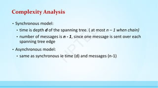
•Figure 4.3 shows an example of vector clocks progress with the increment
value d=1.
•Initially, a vector clock is [0, 0, 0, ...., 0].
N
P
T
E
L

Example of Vector Clock
p 3
p 1
2
0
0
3
0
0
4
3
4
0
1
0
2
0
0 2
3
0
2
4
0
2
3
4
5
3
4
5
6
4
0
0
1
2
3
3
2
3
4
p 2
2
3
0
2
2
0
2
3
2
1
0
0
5
3
4
5
5
4
Figure 4.3: Evolution of vector time.
N
P
T
E
L

Comparing Vector Time Stamps
•The following relations are defined to compare two vector timestamps, vh and vk :
• If the process at which an event occurred is known, the test to compare two
timestamps can be simplified as follows: If events x and y respectively occurred at
processes pi and pj and are assigned timestamps vh and vk, respectively, then
x → y⇔ vh[i ] ≤ vk[i ]
x || y ⇔ vh[i ] > vk[i]∧vh[j ] < vk[j ]
vh = vk ⇔ ∀x : vh[x ] = vk [x ]
vh ≤ vk ⇔ ∀x : vh[x ] ≤ vk [x ]
vh < vk ⇔ vh ≤ vk and ∃x : vh[x ] < vk [x ]
vh || vk ⇔ ¬(vh < vk ) ∧ ¬(vk < vh)
N
P
T
E
L

Properties of Vector Time
Isomorphism
• If events in a distributed system are timestamped using a system of vector
clocks, we have the following property.
• If two events x and y have timestamps vh and vk, respectively, then
x → y ⇔ vh < vk
x || y ⇔ vh || vk
• Thus, there is an isomorphism between the set of partially ordered
events produced by a distributed computation and their vector
timestamps.
N
P
T
E
L

Properties of Vector Time
Strong Consistency
• The system of vector clocks is strongly consistent; thus, by examining the vector
timestamp of two events, we can determine if the events are causally related.
• However, Charron-Bost showed that the dimension of vector clocks cannot be less
than n, the total number of processes in the distributed computation, for this
property to hold.
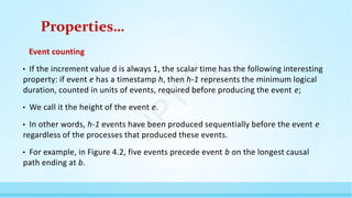
Event Counting
• If d=1 (in rule R1), then the i th component of vector clock at process pi , vti [i ],
denotes the number of events that have occurred at pi until that instant.
• So, if an event e has timestamp vh, vh[j ] denotes the number of events executed by
process pj that causally precede e. Clearly, ∑ vh[j ]− 1 represents the total number
of events that causally precede e in the distributed computation.
N
P
T
E
L

Conclusion
• In a distributed system, a set of processes communicate by exchanging messages
over a communication network. A distributed computation is spread over
geographically distributed processes. The processes do not share a common global
memory or a physical global clock, to which processes have instantaneous access.
• In this lecture we have presented the idea of logical time that was proposed by
Lamport in 1978 in an attempt to order events in distributed systems.
• We have discussed two systems of logical clocks, namely, scalar and vector clocks
to capture causality between events of a distributed computation.
• In upcoming lecture, we will discuss about the size of vector clock, matrix clocks,
virtual time and physical clock synchronization.
N
P
T
E
L

W1_Lecture Notes nptel Distributed system

More Related Content

What's hot

Similar to W1_Lecture Notes nptel Distributed system

Recently uploaded

W1_Lecture Notes nptel Distributed system