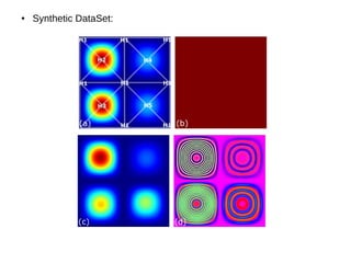
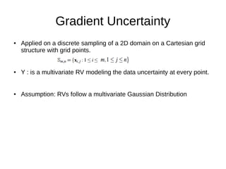
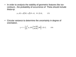
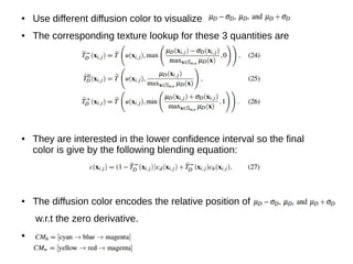
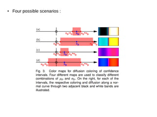
This document summarizes a research paper that presents techniques for visualizing uncertainty in 2D scalar fields. It derives parameters to quantify gradient uncertainty based on data variability. It describes analytical expressions for the probability distributions of gradient magnitude and orientation. A color diffusion technique indicates slope stability, and colored glyphs depict iso-contour uncertainty. The methods are demonstrated on synthetic and seismic ensemble data.

1. Visualizing the Variability of Gradients in
Uncertain 2D Scalar Field
Authors: Tobais Pfaffelmoser, Mihaela Mihai and Rudiger Westermann(TU Munich)
Presented by: Subhashis Hazarika,
The Ohio State University

2. Motivation
● Standard Deviation does not always give a rigorous analysis of
uncertainty, specially when we want to study the differential
quantities, like relative variability of data values at different points.
● To draw inference about the stability of geometric features in a
scalar field like contour shapes.

3. Contribution
● Derivation of gradient based uncertainty parameters on discrete grid
structures.
● Analytical expression of probability distribution describing gradient
magnitude and orientation variation.
● A visualization technique using color diffusion to indicate the stability of
the slope along gradient direction in 2D scalar fields.
● A family of colored glyphs to quantitatively depict the uncertainty in
orientation of iso-contours in 2D scalar fields.

4. Gradient Uncertainty
● Applied on a discrete sampling of a 2D domain on a Cartesian grid
structure with grid points.
● Y : is a multivariate RV modeling the data uncertainty at every point.
● Assumption: RVs follow a multivariate Gaussian Distribution

5. ● Gradient at a point:
● Gradient follows a bivariate Gaussian Distribution whose mean and
covariance is
● The bivariate PDF deltaY for a vector g is :

6. Uncertainty in Derivative
● Choose the mean gradient direction as the direction along which to
determine the uncertainty in derivatives.
● The uncertainty of derivative in the mean gradient direction can be
modeled by a scalar random variable
● RV D must also obey a Gaussian Distribution with mean and
standard deviation:

7. Uncertainty in Orientation
● Convert to polar coordinates:
● Integrating over r (0 to infinity)

8. ● In order to analysis the stability of geometric features like iso-
contours , the probability of occurrence of Theta should include
theta+pi.
● Circular variance to determine the uncertainty in degree of
orientation.

9. Visualization
● To convey the basic shape of the iso-contours in the mean scalar
field they partition the range of mean values into a number of N
equally spaced intervals.

10. ● Use diffusion process to visually encode
● Diffusion at a point takes place along the normal curve, which is the
curve passing through the point and oriented along the gradient
direction.
● Diffusion value : fraction of initial black & white color
● Diffusion value 0.5 implies high degree of diffusion and 1.0 implies
least diffusion.
● Generate a diffusion texture to lookup diffusion value.
● The parameter v(degree of diffusion) is controlled by the gradient
uncertainty parameters.

11. ● Now for a given point the texture coordinates u and v are calculated
as:
● Use a final normalized diffusion value and compute the final color at
each grid point by blending a diffusion color and a background
color.

12. ● Use different diffusion color to visualize
● The corresponding texture lookup for these 3 quantities are
● They are interested in the lower confidence interval so the final
color is give by the following blending equation:
● The diffusion color encodes the relative position of
w.r.t the zero derivative.
●

13. ● Four possible scenarios :

14. Orientation Visualization
● Color of glyph is mapped to the circular variance [0,1] → [ green →
cyan → blue → magenta → red]
● To show individual distribution per glyph the transparency is
controlled at all off-center vertices.
●

15. ● Synthetic DataSet:

16. ● Seismic Ensemble Dataset: