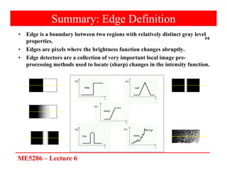
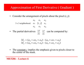
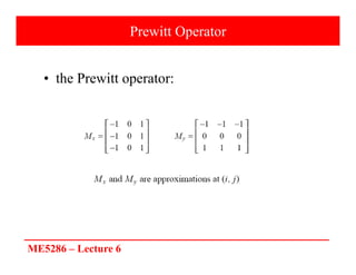
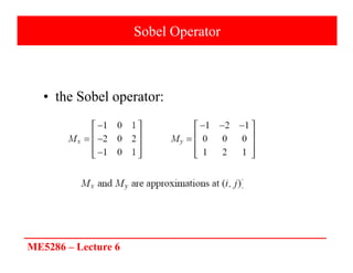
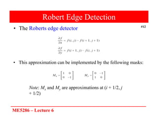
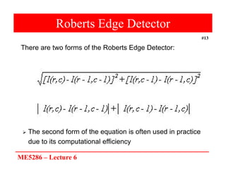
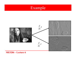
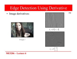
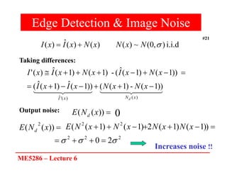
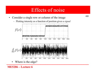
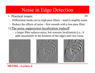
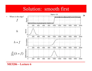
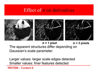
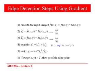
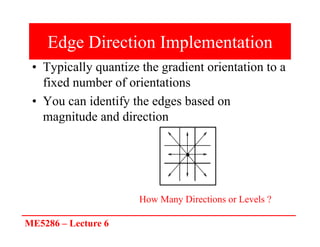
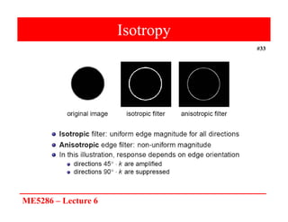
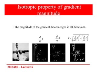
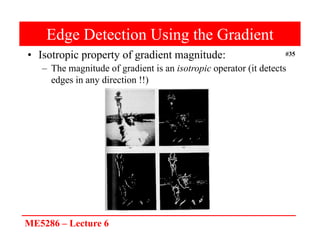
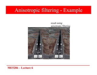
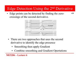
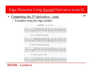
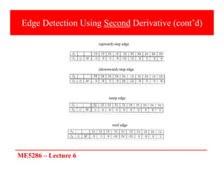
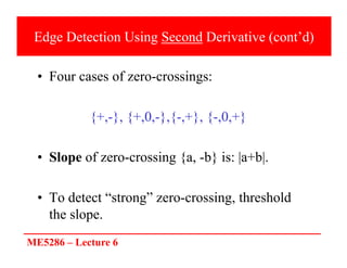
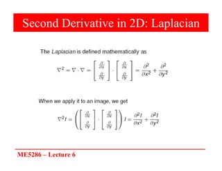
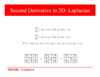
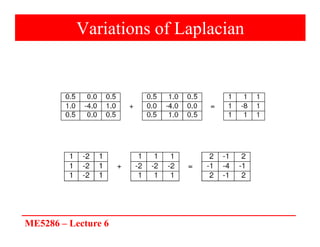
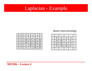
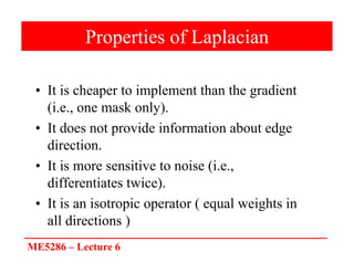
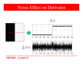
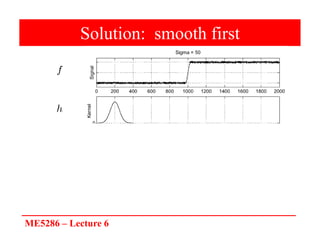
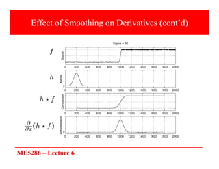
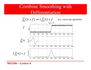
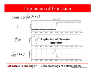
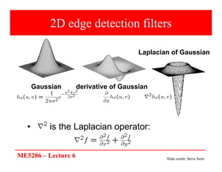
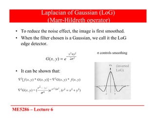
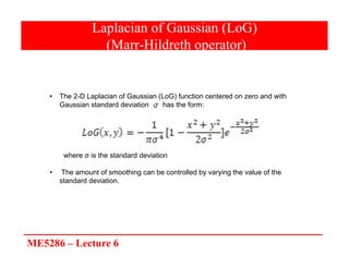
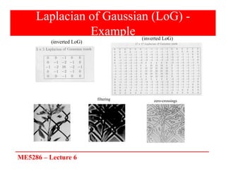
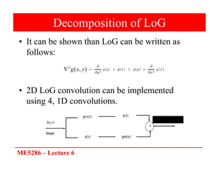
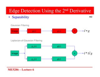
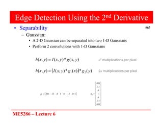
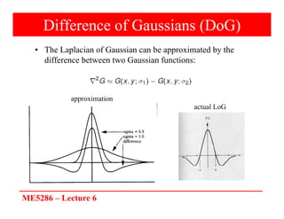
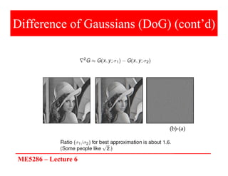
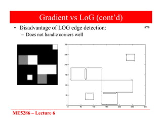
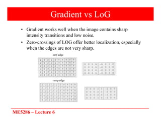
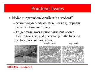
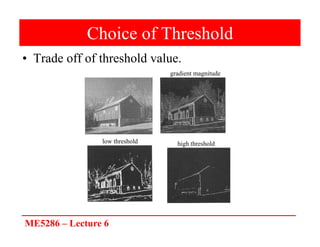
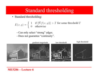
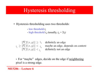
ME5286 – Lecture 6
#1
Lecture 7:
Edge Detection
Saad J Bedros
sbedros@umn.edu
ME5286 – Lecture 6
#2
Review From Last Lecture
• Definition of an Edge
• First Order Derivative Approximation as
Edge Detector
ME5286 – Lecture 6
#3
This Lecture
• Examples of Edge Detection with first order
derivative approximation
• Edge Detection with Second order
derivative
• Combining Smoothing and Edge Detection
with Laplacian of Gaussian
ME5286 – Lecture 6
#4
Summary: Edge Definition
• Edge is a boundary between two regions with relatively distinct gray level
properties.
• Edges are pixels where the brightness function changes abruptly.
• Edge detectors are a collection of very important local image pre-
processing methods used to locate (sharp) changes in the intensity function.
ME5286 – Lecture 6
Criteria for Optimal Edge Detection
• (1) Good detection
– Minimize the probability of false positives (i.e., spurious edges).
– Minimize the probability of false negatives (i.e., missing real
edges).
• (2) Good localization
– Detected edges must be as close as possible to the true edges.
• (3) Single response
– Minimize the number of local maxima around the true edge.
ME5286 – Lecture 6
Edge Detection Using Derivatives
• Often, points that lie on an edge
are detected by:
(1) Detecting the local maxima or
minima of the first derivative.
(2) Detecting the zero-crossings
of the second derivative.
2nd derivative
1st derivative
ME5286 – Lecture 6
Edge Detection Using First Derivative
sensitive to vertical edges!
sensitive to horizontal edges!
ME5286 – Lecture 6
• We can implement and using the following masks:
(x+1/2,y)
(x,y+1/2)
*
*
good approximation
at (x+1/2,y)
good approximation
at (x,y+1/2)
Edge Detection Using First Derivative
ME5286 – Lecture 6
Approximation of First Derivative ( Gradient )
• Consider the arrangement of pixels about the pixel (i, j):
• The partial derivatives can be computed by:
• The constant c implies the emphasis given to pixels closer to
the center of the mask.
3 x 3 neighborhood:
ME5286 – Lecture 6
Prewitt Operator
• the Prewitt operator:
ME5286 – Lecture 6
Sobel Operator
• the Sobel operator:
ME5286 – Lecture 6
#12
Robert Edge Detection
• The Roberts edge detector
• This approximation can be implemented by the following masks:
Note: Mx and My are approximations at (i + 1/2, j
+ 1/2)
ME5286 – Lecture 6
#13
Roberts Edge Detector
There are two forms of the Roberts Edge Detector:
 The second form of the equation is often used in practice
due to its computational efficiency
ME5286 – Lecture 6
#14
Roberts Edge Detector
• A simple approximation to the first
derivative
• Marks edge points only; it does not return
any information about the edge
orientation
• Simplest of the edge detection operators
and will work best with binary images
ME5286 – Lecture 6
Example
I
dx
d
I
dy
d
ME5286 – Lecture 6
#16
Edge Detection Using Derivative
• Image derivatives:
 
1
1
* 
 I
Ix







1
1
*
I
Iy
Image I
ME5286 – Lecture 6
#17
Edge Detection Using the Gradient
• Example – cont.:
2
2
















 I
dy
d
I
dx
d
ME5286 – Lecture 6
#18
Edge Detection Using the Gradient
• Example – cont.:
100


 Threshold
ME5286 – Lecture 6
#19
Derivatives and Noise
• Derivatives are strongly affected by noise
– obvious reason: image noise results in pixels that look very
different from their neighbors
– The larger the noise - the stronger the response
• What is to be done?
– Neighboring pixels look alike
– Pixel along an edge look alike
– Image smoothing should help
– Force pixels different to their neighbors (possibly noise) to
look like neighbors
ME5286 – Lecture 6
#20
Derivatives and Noise
Increasing noise
– Need to perform image smoothing as a preliminary step
– Generally – use Gaussian smoothing
ME5286 – Lecture 6
#21
Edge Detection & Image Noise
i.i.d
)
,
0
(
~
)
(
)
(
)
(
ˆ
)
( 
N
x
N
x
N
x
I
x
I 



 


 



 


 

)
(
)
(
'
ˆ
))
1
(
-
)
1
(
(
))
1
(
ˆ
)
1
(
ˆ
(
))
1
(
)
1
(
ˆ
(
-
)
1
(
)
1
(
ˆ
)
(
'
x
N
x
I d
x
N
x
N
x
I
x
I
x
N
x
I
x
N
x
I
x
I
















))
(
( x
N
E d 0
Taking differences:
Output noise:

))
(
(
2
x
N
E d






 )
)
1
(
)
1
(
2
)
1
(
)
1
(
( 2
2
x
N
x
N
x
N
x
N
E
2
2
2
2
0 

 



Increases noise !!
ME5286 – Lecture 6
#22
Effects of noise
• Consider a single row or column of the image
– Plotting intensity as a function of position gives a signal
• Where is the edge?
ME5286 – Lecture 6
#23
Noise in Edge Detection
• Practical issues:
– Differential masks act as high-pass filters – tend to amplify noise.
– Reduce the effects of noise - first smooth with a low-pass filter.
1)The noise suppression-localization tradeoff
– a larger filter reduces noise, but worsens localization (i.e., it
adds uncertainty to the location of the edge) and vice-versa.
ME5286 – Lecture 6
#24
• Where is the edge?
Solution: smooth first
ME5286 – Lecture 6
#25
Derivative theorem of convolution
• This saves us one operation:
ME5286 – Lecture 6
 
1
1 

0.0030 0.0133 0.0219 0.0133 0.0030
0.0133 0.0596 0.0983 0.0596 0.0133
0.0219 0.0983 0.1621 0.0983 0.0219
0.0133 0.0596 0.0983 0.0596 0.0133
0.0030 0.0133 0.0219 0.0133 0.0030
)
(
)
( h
g
I
h
g
I 




Derivative of Gaussian filters
ME5286 – Lecture 6
Derivative of Gaussian filters
x-direction y-direction
Source: L. Lazebnik
ME5286 – Lecture 6
Smoothing with a Gaussian
Recall: parameter σ is the “scale” / “width” / “spread” of the
Gaussian kernel, and controls the amount of smoothing.
…
ME5286 – Lecture 6
Effect of σ on derivatives
The apparent structures differ depending on
Gaussian’s scale parameter.
Larger values: larger scale edges detected
Smaller values: finer features detected
σ = 1 pixel σ = 3 pixels
ME5286 – Lecture 6
Edge Detection Steps Using Gradient
(i.e., sqrt is costly!)
ME5286 – Lecture 6
Edge Direction Implementation
• Typically quantize the gradient orientation to a
fixed number of orientations
• You can identify the edges based on
magnitude and direction
How Many Directions or Levels ?
ME5286 – Lecture 6
#32
ME5286 – Lecture 6
Isotropy
#33
ME5286 – Lecture 6
Isotropic property of gradient
magnitude
• The magnitude of the gradient detects edges in all directions.
2
2
d d
I I
dx dy
 
 
    
 
   
I
dx
d I
dy
d
ME5286 – Lecture 6
#35
Edge Detection Using the Gradient
• Isotropic property of gradient magnitude:
– The magnitude of gradient is an isotropic operator (it detects
edges in any direction !!)
ME5286 – Lecture 6
Anisotropic Filtering
(i.e., edge preserving smoothing)
• Symmetric Gaussian smoothing tends to blur out edges
rather aggressively.
• An “oriented” smoothing operator would work better:
(i) Smooth aggressively perpendicular to the gradient
(ii) Smooth little along the gradient
ME5286 – Lecture 6
Anisotropic filtering - Example
result using
anisotropic filtering
ME5286 – Lecture 6
#38
ME5286 – Lecture 6
#39
Edge Detection Using the 2nd Derivative
• Edge points can be detected by finding the zero-
crossings of the second derivative.
• There are two approaches that uses the second
derivative to identify the edge presence
• Smoothing then apply Gradient
• Combine smoothing and Gradient Opertations
ME5286 – Lecture 6
Edge Detection Using Second
Derivative
• Approximate finding maxima/minima of
gradient magnitude by finding places
where:
• Can’t always find discrete pixels where the
second derivative is zero – look for zero-
crossing instead.
ME5286 – Lecture 6
#41
Edge Detection Using Second Derivative
• Computing the 2nd derivative:
– This approximation is centered about x + 1
– By replacing x + 1 by x we obtain:
ME5286 – Lecture 6
Image Derivatives
• 1st order
• 2nd order
ME5286 – Lecture 6
Edge Detection Using Second Derivative (cont’d)
ME5286 – Lecture 6
#44
Edge Detection Using Second Derivative (cont’d)
• Computing the 2nd derivative – cont.
– Examples using the edge models:
ME5286 – Lecture 6
Edge Detection Using Second Derivative (cont’d)
(upward) step edge
(downward) step edge
ramp edge
roof edge
ME5286 – Lecture 6
Edge Detection Using Second Derivative (cont’d)
• Four cases of zero-crossings:
{+,-}, {+,0,-},{-,+}, {-,0,+}
• Slope of zero-crossing {a, -b} is: |a+b|.
• To detect “strong” zero-crossing, threshold
the slope.
ME5286 – Lecture 6
Second Derivative in 2D: Laplacian
ME5286 – Lecture 6
Second Derivative in 2D: Laplacian
ME5286 – Lecture 6
Variations of Laplacian
ME5286 – Lecture 6
Laplacian - Example
detect zero-crossings
ME5286 – Lecture 6
Properties of Laplacian
• It is cheaper to implement than the gradient
(i.e., one mask only).
• It does not provide information about edge
direction.
• It is more sensitive to noise (i.e.,
differentiates twice).
• It is an isotropic operator ( equal weights in
all directions )
ME5286 – Lecture 6
Noise Effect on Derivates
Where is the edge??
ME5286 – Lecture 6
Solution: smooth first
ME5286 – Lecture 6
Effect of Smoothing on Derivatives (cont’d)
ME5286 – Lecture 6
Combine Smoothing with
Differentiation
(i.e., saves one operation)
ME5286 – Lecture 6
Laplacian of Gaussian
Consider
Laplacian of Gaussian
operator
Where is the edge? Zero-crossings of bottom graph
Slide credit: Steve Seitz
ME5286 – Lecture 6
2D edge detection filters
• is the Laplacian operator:
Laplacian of Gaussian
Gaussian derivative of Gaussian
Slide credit: Steve Seitz
ME5286 – Lecture 6
Laplacian of Gaussian (LoG)
(Marr-Hildreth operator)
• To reduce the noise effect, the image is first smoothed.
• When the filter chosen is a Gaussian, we call it the LoG
edge detector.
• It can be shown that:
σ controls smoothing
2σ2
(inverted
LoG)
ME5286 – Lecture 6
Laplacian of Gaussian (LoG)
(Marr-Hildreth operator)
• The 2-D Laplacian of Gaussian (LoG) function centered on zero and with
Gaussian standard deviation has the form:
where σ is the standard deviation
• The amount of smoothing can be controlled by varying the value of the
standard deviation.
ME5286 – Lecture 6
Laplacian of Gaussian (LoG) -
Example
filtering zero-crossings
(inverted LoG)
(inverted LoG)
ME5286 – Lecture 6
Decomposition of LoG
• It can be shown than LoG can be written as
follows:
• 2D LoG convolution can be implemented
using 4, 1D convolutions.
2
( , )
g x y

2
( , )* ( , )
g x y I x y

ME5286 – Lecture 6
#62
Edge Detection Using the 2nd Derivative
• Separability
Image
gxx(x) g(x)
gyy(y) g(y)
+ g
I 2
*
Image g(x) g(y) + g
I 
Gaussian Filtering
Laplacian-of-Gaussian Filtering
ME5286 – Lecture 6
#63
Edge Detection Using the 2nd Derivative
• Separability
– Gaussian:
• A 2-D Gaussian can be separated into two 1-D Gaussians
• Perform 2 convolutions with 1-D Gaussians
)
,
(
*
)
,
(
)
,
( y
x
g
y
x
I
y
x
h 
  )
(
*
)
(
*
)
,
(
)
,
( 2
1 y
g
x
g
y
x
I
y
x
h 
n2 multiplications per pixel
2n multiplications per pixel
 
011
.
13
.
6
.
1
6
.
13
.
011
.
1 
g























011
.
13
.
6
.
1
6
.
13
.
011
.
2
g
ME5286 – Lecture 6
Decomposition of LoG (cont’d)
Steps
ME5286 – Lecture 6
#65
Edge Detection Using LOG
• Marr-Hildteth (LOG) Algorithm:
– Compute LoG
• Use one 2D filter:
• Use four 1D filters:
– Find zero-crossings from each row and column
– Find slope of zero-crossings
– Apply threshold to slope and mark edges
)
,
(
2
y
x
g

)
(
),
(
),
(
),
( y
g
y
g
x
g
x
g yy
xx
ME5286 – Lecture 6
#66
Laplacian of Gaussian (LoG) - Example
• The Laplacian-of-Gaussian (LOG) – cont.
 
G
I 2
* 
I
)
(
*
I
of
crossings
Zero 2
G

ME5286 – Lecture 6
#67
Laplacian of Gaussian (LoG) - Example
• The Laplacian-of-Gaussian (LOG) – cont.
1


6


3


ME5286 – Lecture 6
Difference of Gaussians (DoG)
• The Laplacian of Gaussian can be approximated by the
difference between two Gaussian functions:
approximation
actual LoG
ME5286 – Lecture 6
Difference of Gaussians (DoG) (cont’d)
(a) (b) (b)‐(a)
ME5286 – Lecture 6
#70
Gradient vs LoG (cont’d)
• Disadvantage of LOG edge detection:
– Does not handle corners well
ME5286 – Lecture 6
Gradient vs LoG
• Gradient works well when the image contains sharp
intensity transitions and low noise.
• Zero-crossings of LOG offer better localization, especially
when the edges are not very sharp.
step edge
ramp edge
ME5286 – Lecture 6
Practical Issues
• Noise suppression-localization tradeoff.
– Smoothing depends on mask size (e.g., depends
on σ for Gaussian filters).
– Larger mask sizes reduce noise, but worsen
localization (i.e., add uncertainty to the location
of the edge) and vice versa.
larger mask
smaller mask
ME5286 – Lecture 6
Choice of Threshold
• Trade off of threshold value.
gradient magnitude
low threshold high threshold
ME5286 – Lecture 6
Standard thresholding
• Standard thresholding:
- Can only select “strong” edges.
- Does not guarantee “continuity”.
gradient magnitude low threshold high threshold
ME5286 – Lecture 6
Hysteresis thresholding
• Hysteresis thresholding uses two thresholds:
• For “maybe” edges, decide on the edge if neighboring
pixel is a strong edge.
- low threshold tl
- high threshold th (usually, th = 2tl)
tl
tl
th
th
ME5286 – Lecture 6
Hysteresis Thresholding Example
#76
ME5286 – Lecture 6
#77
Edge Detection Review
• Edge detection operators are based on the idea that
edge information in an image is found by looking
at the relationship a pixel has with its neighbors
• If a pixel's gray level value is similar to those
around it, there is probably not an edge at that
point
ME5286 – Lecture 6
#78
Edge Detection Review
• Edge detection operators are often
implemented with convolution masks and
most are based on discrete approximations
to differential operators
• Differential operations measure the rate of
change in a function, in this case, the image
brightness function
ME5286 – Lecture 6
#79
Edge Detection Review
• Preprocessing of image is required to eliminate or
at least minimize noise effects
• There is tradeoff between sensitivity and accuracy
in edge detection
• The parameters that we can set so that edge
detector is sensitive include the size of the edge
detection mask and the value of the gray level
threshold
• A larger mask or a higher gray level threshold will
tend to reduce noise effects, but may result in a
loss of valid edge points

Edge Detection 2 digital image processing

  • 1.
    ME5286 – Lecture6 #1 Lecture 7: Edge Detection Saad J Bedros sbedros@umn.edu
  • 2.
    ME5286 – Lecture6 #2 Review From Last Lecture • Definition of an Edge • First Order Derivative Approximation as Edge Detector
  • 3.
    ME5286 – Lecture6 #3 This Lecture • Examples of Edge Detection with first order derivative approximation • Edge Detection with Second order derivative • Combining Smoothing and Edge Detection with Laplacian of Gaussian
  • 4.
    ME5286 – Lecture6 #4 Summary: Edge Definition • Edge is a boundary between two regions with relatively distinct gray level properties. • Edges are pixels where the brightness function changes abruptly. • Edge detectors are a collection of very important local image pre- processing methods used to locate (sharp) changes in the intensity function.
  • 5.
    ME5286 – Lecture6 Criteria for Optimal Edge Detection • (1) Good detection – Minimize the probability of false positives (i.e., spurious edges). – Minimize the probability of false negatives (i.e., missing real edges). • (2) Good localization – Detected edges must be as close as possible to the true edges. • (3) Single response – Minimize the number of local maxima around the true edge.
  • 6.
    ME5286 – Lecture6 Edge Detection Using Derivatives • Often, points that lie on an edge are detected by: (1) Detecting the local maxima or minima of the first derivative. (2) Detecting the zero-crossings of the second derivative. 2nd derivative 1st derivative
  • 7.
    ME5286 – Lecture6 Edge Detection Using First Derivative sensitive to vertical edges! sensitive to horizontal edges!
  • 8.
    ME5286 – Lecture6 • We can implement and using the following masks: (x+1/2,y) (x,y+1/2) * * good approximation at (x+1/2,y) good approximation at (x,y+1/2) Edge Detection Using First Derivative
  • 9.
    ME5286 – Lecture6 Approximation of First Derivative ( Gradient ) • Consider the arrangement of pixels about the pixel (i, j): • The partial derivatives can be computed by: • The constant c implies the emphasis given to pixels closer to the center of the mask. 3 x 3 neighborhood:
  • 10.
    ME5286 – Lecture6 Prewitt Operator • the Prewitt operator:
  • 11.
    ME5286 – Lecture6 Sobel Operator • the Sobel operator:
  • 12.
    ME5286 – Lecture6 #12 Robert Edge Detection • The Roberts edge detector • This approximation can be implemented by the following masks: Note: Mx and My are approximations at (i + 1/2, j + 1/2)
  • 13.
    ME5286 – Lecture6 #13 Roberts Edge Detector There are two forms of the Roberts Edge Detector:  The second form of the equation is often used in practice due to its computational efficiency
  • 14.
    ME5286 – Lecture6 #14 Roberts Edge Detector • A simple approximation to the first derivative • Marks edge points only; it does not return any information about the edge orientation • Simplest of the edge detection operators and will work best with binary images
  • 15.
    ME5286 – Lecture6 Example I dx d I dy d
  • 16.
    ME5286 – Lecture6 #16 Edge Detection Using Derivative • Image derivatives:   1 1 *   I Ix        1 1 * I Iy Image I
  • 17.
    ME5286 – Lecture6 #17 Edge Detection Using the Gradient • Example – cont.: 2 2                  I dy d I dx d
  • 18.
    ME5286 – Lecture6 #18 Edge Detection Using the Gradient • Example – cont.: 100    Threshold
  • 19.
    ME5286 – Lecture6 #19 Derivatives and Noise • Derivatives are strongly affected by noise – obvious reason: image noise results in pixels that look very different from their neighbors – The larger the noise - the stronger the response • What is to be done? – Neighboring pixels look alike – Pixel along an edge look alike – Image smoothing should help – Force pixels different to their neighbors (possibly noise) to look like neighbors
  • 20.
    ME5286 – Lecture6 #20 Derivatives and Noise Increasing noise – Need to perform image smoothing as a preliminary step – Generally – use Gaussian smoothing
  • 21.
    ME5286 – Lecture6 #21 Edge Detection & Image Noise i.i.d ) , 0 ( ~ ) ( ) ( ) ( ˆ ) (  N x N x N x I x I                     ) ( ) ( ' ˆ )) 1 ( - ) 1 ( ( )) 1 ( ˆ ) 1 ( ˆ ( )) 1 ( ) 1 ( ˆ ( - ) 1 ( ) 1 ( ˆ ) ( ' x N x I d x N x N x I x I x N x I x N x I x I                 )) ( ( x N E d 0 Taking differences: Output noise:  )) ( ( 2 x N E d        ) ) 1 ( ) 1 ( 2 ) 1 ( ) 1 ( ( 2 2 x N x N x N x N E 2 2 2 2 0        Increases noise !!
  • 22.
    ME5286 – Lecture6 #22 Effects of noise • Consider a single row or column of the image – Plotting intensity as a function of position gives a signal • Where is the edge?
  • 23.
    ME5286 – Lecture6 #23 Noise in Edge Detection • Practical issues: – Differential masks act as high-pass filters – tend to amplify noise. – Reduce the effects of noise - first smooth with a low-pass filter. 1)The noise suppression-localization tradeoff – a larger filter reduces noise, but worsens localization (i.e., it adds uncertainty to the location of the edge) and vice-versa.
  • 24.
    ME5286 – Lecture6 #24 • Where is the edge? Solution: smooth first
  • 25.
    ME5286 – Lecture6 #25 Derivative theorem of convolution • This saves us one operation:
  • 26.
    ME5286 – Lecture6   1 1   0.0030 0.0133 0.0219 0.0133 0.0030 0.0133 0.0596 0.0983 0.0596 0.0133 0.0219 0.0983 0.1621 0.0983 0.0219 0.0133 0.0596 0.0983 0.0596 0.0133 0.0030 0.0133 0.0219 0.0133 0.0030 ) ( ) ( h g I h g I      Derivative of Gaussian filters
  • 27.
    ME5286 – Lecture6 Derivative of Gaussian filters x-direction y-direction Source: L. Lazebnik
  • 28.
    ME5286 – Lecture6 Smoothing with a Gaussian Recall: parameter σ is the “scale” / “width” / “spread” of the Gaussian kernel, and controls the amount of smoothing. …
  • 29.
    ME5286 – Lecture6 Effect of σ on derivatives The apparent structures differ depending on Gaussian’s scale parameter. Larger values: larger scale edges detected Smaller values: finer features detected σ = 1 pixel σ = 3 pixels
  • 30.
    ME5286 – Lecture6 Edge Detection Steps Using Gradient (i.e., sqrt is costly!)
  • 31.
    ME5286 – Lecture6 Edge Direction Implementation • Typically quantize the gradient orientation to a fixed number of orientations • You can identify the edges based on magnitude and direction How Many Directions or Levels ?
  • 32.
  • 33.
    ME5286 – Lecture6 Isotropy #33
  • 34.
    ME5286 – Lecture6 Isotropic property of gradient magnitude • The magnitude of the gradient detects edges in all directions. 2 2 d d I I dx dy                I dx d I dy d
  • 35.
    ME5286 – Lecture6 #35 Edge Detection Using the Gradient • Isotropic property of gradient magnitude: – The magnitude of gradient is an isotropic operator (it detects edges in any direction !!)
  • 36.
    ME5286 – Lecture6 Anisotropic Filtering (i.e., edge preserving smoothing) • Symmetric Gaussian smoothing tends to blur out edges rather aggressively. • An “oriented” smoothing operator would work better: (i) Smooth aggressively perpendicular to the gradient (ii) Smooth little along the gradient
  • 37.
    ME5286 – Lecture6 Anisotropic filtering - Example result using anisotropic filtering
  • 38.
  • 39.
    ME5286 – Lecture6 #39 Edge Detection Using the 2nd Derivative • Edge points can be detected by finding the zero- crossings of the second derivative. • There are two approaches that uses the second derivative to identify the edge presence • Smoothing then apply Gradient • Combine smoothing and Gradient Opertations
  • 40.
    ME5286 – Lecture6 Edge Detection Using Second Derivative • Approximate finding maxima/minima of gradient magnitude by finding places where: • Can’t always find discrete pixels where the second derivative is zero – look for zero- crossing instead.
  • 41.
    ME5286 – Lecture6 #41 Edge Detection Using Second Derivative • Computing the 2nd derivative: – This approximation is centered about x + 1 – By replacing x + 1 by x we obtain:
  • 42.
    ME5286 – Lecture6 Image Derivatives • 1st order • 2nd order
  • 43.
    ME5286 – Lecture6 Edge Detection Using Second Derivative (cont’d)
  • 44.
    ME5286 – Lecture6 #44 Edge Detection Using Second Derivative (cont’d) • Computing the 2nd derivative – cont. – Examples using the edge models:
  • 45.
    ME5286 – Lecture6 Edge Detection Using Second Derivative (cont’d) (upward) step edge (downward) step edge ramp edge roof edge
  • 46.
    ME5286 – Lecture6 Edge Detection Using Second Derivative (cont’d) • Four cases of zero-crossings: {+,-}, {+,0,-},{-,+}, {-,0,+} • Slope of zero-crossing {a, -b} is: |a+b|. • To detect “strong” zero-crossing, threshold the slope.
  • 47.
    ME5286 – Lecture6 Second Derivative in 2D: Laplacian
  • 48.
    ME5286 – Lecture6 Second Derivative in 2D: Laplacian
  • 49.
    ME5286 – Lecture6 Variations of Laplacian
  • 50.
    ME5286 – Lecture6 Laplacian - Example detect zero-crossings
  • 51.
    ME5286 – Lecture6 Properties of Laplacian • It is cheaper to implement than the gradient (i.e., one mask only). • It does not provide information about edge direction. • It is more sensitive to noise (i.e., differentiates twice). • It is an isotropic operator ( equal weights in all directions )
  • 52.
    ME5286 – Lecture6 Noise Effect on Derivates Where is the edge??
  • 53.
    ME5286 – Lecture6 Solution: smooth first
  • 54.
    ME5286 – Lecture6 Effect of Smoothing on Derivatives (cont’d)
  • 55.
    ME5286 – Lecture6 Combine Smoothing with Differentiation (i.e., saves one operation)
  • 56.
    ME5286 – Lecture6 Laplacian of Gaussian Consider Laplacian of Gaussian operator Where is the edge? Zero-crossings of bottom graph Slide credit: Steve Seitz
  • 57.
    ME5286 – Lecture6 2D edge detection filters • is the Laplacian operator: Laplacian of Gaussian Gaussian derivative of Gaussian Slide credit: Steve Seitz
  • 58.
    ME5286 – Lecture6 Laplacian of Gaussian (LoG) (Marr-Hildreth operator) • To reduce the noise effect, the image is first smoothed. • When the filter chosen is a Gaussian, we call it the LoG edge detector. • It can be shown that: σ controls smoothing 2σ2 (inverted LoG)
  • 59.
    ME5286 – Lecture6 Laplacian of Gaussian (LoG) (Marr-Hildreth operator) • The 2-D Laplacian of Gaussian (LoG) function centered on zero and with Gaussian standard deviation has the form: where σ is the standard deviation • The amount of smoothing can be controlled by varying the value of the standard deviation.
  • 60.
    ME5286 – Lecture6 Laplacian of Gaussian (LoG) - Example filtering zero-crossings (inverted LoG) (inverted LoG)
  • 61.
    ME5286 – Lecture6 Decomposition of LoG • It can be shown than LoG can be written as follows: • 2D LoG convolution can be implemented using 4, 1D convolutions. 2 ( , ) g x y  2 ( , )* ( , ) g x y I x y 
  • 62.
    ME5286 – Lecture6 #62 Edge Detection Using the 2nd Derivative • Separability Image gxx(x) g(x) gyy(y) g(y) + g I 2 * Image g(x) g(y) + g I  Gaussian Filtering Laplacian-of-Gaussian Filtering
  • 63.
    ME5286 – Lecture6 #63 Edge Detection Using the 2nd Derivative • Separability – Gaussian: • A 2-D Gaussian can be separated into two 1-D Gaussians • Perform 2 convolutions with 1-D Gaussians ) , ( * ) , ( ) , ( y x g y x I y x h    ) ( * ) ( * ) , ( ) , ( 2 1 y g x g y x I y x h  n2 multiplications per pixel 2n multiplications per pixel   011 . 13 . 6 . 1 6 . 13 . 011 . 1  g                        011 . 13 . 6 . 1 6 . 13 . 011 . 2 g
  • 64.
    ME5286 – Lecture6 Decomposition of LoG (cont’d) Steps
  • 65.
    ME5286 – Lecture6 #65 Edge Detection Using LOG • Marr-Hildteth (LOG) Algorithm: – Compute LoG • Use one 2D filter: • Use four 1D filters: – Find zero-crossings from each row and column – Find slope of zero-crossings – Apply threshold to slope and mark edges ) , ( 2 y x g  ) ( ), ( ), ( ), ( y g y g x g x g yy xx
  • 66.
    ME5286 – Lecture6 #66 Laplacian of Gaussian (LoG) - Example • The Laplacian-of-Gaussian (LOG) – cont.   G I 2 *  I ) ( * I of crossings Zero 2 G 
  • 67.
    ME5286 – Lecture6 #67 Laplacian of Gaussian (LoG) - Example • The Laplacian-of-Gaussian (LOG) – cont. 1   6   3  
  • 68.
    ME5286 – Lecture6 Difference of Gaussians (DoG) • The Laplacian of Gaussian can be approximated by the difference between two Gaussian functions: approximation actual LoG
  • 69.
    ME5286 – Lecture6 Difference of Gaussians (DoG) (cont’d) (a) (b) (b)‐(a)
  • 70.
    ME5286 – Lecture6 #70 Gradient vs LoG (cont’d) • Disadvantage of LOG edge detection: – Does not handle corners well
  • 71.
    ME5286 – Lecture6 Gradient vs LoG • Gradient works well when the image contains sharp intensity transitions and low noise. • Zero-crossings of LOG offer better localization, especially when the edges are not very sharp. step edge ramp edge
  • 72.
    ME5286 – Lecture6 Practical Issues • Noise suppression-localization tradeoff. – Smoothing depends on mask size (e.g., depends on σ for Gaussian filters). – Larger mask sizes reduce noise, but worsen localization (i.e., add uncertainty to the location of the edge) and vice versa. larger mask smaller mask
  • 73.
    ME5286 – Lecture6 Choice of Threshold • Trade off of threshold value. gradient magnitude low threshold high threshold
  • 74.
    ME5286 – Lecture6 Standard thresholding • Standard thresholding: - Can only select “strong” edges. - Does not guarantee “continuity”. gradient magnitude low threshold high threshold
  • 75.
    ME5286 – Lecture6 Hysteresis thresholding • Hysteresis thresholding uses two thresholds: • For “maybe” edges, decide on the edge if neighboring pixel is a strong edge. - low threshold tl - high threshold th (usually, th = 2tl) tl tl th th
  • 76.
    ME5286 – Lecture6 Hysteresis Thresholding Example #76
  • 77.
    ME5286 – Lecture6 #77 Edge Detection Review • Edge detection operators are based on the idea that edge information in an image is found by looking at the relationship a pixel has with its neighbors • If a pixel's gray level value is similar to those around it, there is probably not an edge at that point
  • 78.
    ME5286 – Lecture6 #78 Edge Detection Review • Edge detection operators are often implemented with convolution masks and most are based on discrete approximations to differential operators • Differential operations measure the rate of change in a function, in this case, the image brightness function
  • 79.
    ME5286 – Lecture6 #79 Edge Detection Review • Preprocessing of image is required to eliminate or at least minimize noise effects • There is tradeoff between sensitivity and accuracy in edge detection • The parameters that we can set so that edge detector is sensitive include the size of the edge detection mask and the value of the gray level threshold • A larger mask or a higher gray level threshold will tend to reduce noise effects, but may result in a loss of valid edge points