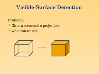
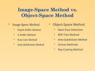
Visible surface detection methods, also known as hidden surface removal algorithms, are techniques used in computer graphics to determine which surfaces of 3D objects are visible from a specific viewpoint. These methods are crucial for creating realistic images by ensuring that only the visible portions of objects are displayed, hiding surfaces that are obstructed by others.

1. Visible-Surface Detection Methods

2. Contents
 Abstract
 Introduction
 Back-Face Detection
 Depth-Buffer Method
 A-Buffer Method
 Scan-Line Method
 Depth-Sorting Method
 BSP-Tree Method
 Area-Subdivision Method
 Octree Method
 Ray-Casting Method
 Image-Space Method vs.
Object-Space Method
 Curved Surfaces
 Wireframe Methods
 Summary

3. Abstract
 Hidden-surface elimination methods
 Identifying visible parts of a scene from a viewpoint
 Numerous algorithms
• More memory - storage
• More processing time – execution time
• Only for special types of objects - constraints
 Deciding a method for a particular application
• Complexity of the scene
• Type of objects
• Available equipment
• Static or animated scene
<Ex. Wireframe Displays>

4. Visible-Surface Detection
Problem:
 Given a scene and a projection,
 what can we see?

5. Visible-Surface Detection …
Terminology:
 Visible-surface detection vs. hidden-surface removal
 Hidden-line removal vs. hidden-surface removal
Many algorithms:
• Complexity scene
• Type of objects
• Hardware

6. Visible-Surface Detection …
Two main types of algorithms:
 Object space: Determine which part of the object are visible
 Image space: Determine per pixel which point of an object is visible
Object space Image space

7. Visible-Surface Detection …
Visible-surface detection = sort for depth
• what and in what order varies
Performance: use coherence
• Objects
• Position in world space
• Position in image space
• Time
Note : Coherence is the result of local similarity

8. Introduction

9. Classification of
Visible-Surface Detection Algorithms
 Object-space methods vs. Image-space methods
• Object definition directly vs. their projected images
• Most visible-surface algorithms use image-space methods
• Object-space can be used effectively in some cases
 Ex: Line-display algorithms
 Object-space methods
• Compares objects and parts of objects to each other
 Image-space methods
• Point by point at each pixel position on the projection plane

10. Sorting and Coherence Methods
 To improve performance
 Sorting
• Facilitate depth comparisons
 Ordering the surfaces according to their distance from the viewplane
 Coherence
• Take advantage of regularity
 Epipolar geometry
 Topological coherence

11. Back-Face Detection

12. Inside-outside test
 A point (x, y, z) is “inside” a surface with plane
parameters A, B, C, and D if
 The polygon is a back face if
• V is a vector in the viewing direction from the eye(camera)
• N is the normal vector to a polygon surface
0



 D
Cz
By
Ax
0

N
V V
N = (A, B, C)

13. Advanced Configuration
 In the case of concave polyhedron
• Need more tests
 Determine faces totally or partly obscured by other faces
• In general, back-face removal can be expected to eliminate about half of
the surfaces from further visibility tests
<View of a concave polyhedron with
one face partially hidden by other surfaces>

14. Depth-Buffer Method
(Z-Buffer Method)
 It is a commonly used image-space approach to detecting
visible surfaces proposed by CatMullin 1974.
 It compares the surface depths at each pixel position on
the projection plane.
 Object depth is usually measured from the view plane
along the z axis of a viewing system.
 Each surface of a scene is processed separately, one point
at a time across the surface.

15. Depth-Buffer Method :
Characteristics
 Commonly used image-space approach
 Compares depths of each pixel on the projection plane
• Referred to as the z-buffer method
 Usually applied to scenes of polygonal surfaces
• Depth values can be computed very quickly
• Easy to implement
Yv
Xv
Zv
S1
S2
S3
(x, y)

16. Depth-Buffer Method :
Depth Buffer & Refresh Buffer
 Two buffer areas are required
• Depth buffer
 Store depth values for each (x, y) position
 0 ≤ depth ≤ 1
 All positions are initialized to minimum depth
 Usually 0 – most distant depth from the viewplane
• Refresh buffer
 Stores the intensity values for each position
 All positions are initialized to the background intensity

17. Depth-Buffer Method :
Algorithm
 Initialize the depth buffer and refresh buffer
depth(x, y) = 0, refresh(x, y) = Ibackgnd
 For each position on each polygon surface
• Calculate the depth for each (x, y) position on the polygon
• If z > depth(x, y), then set
depth(x, y) = z, refresh(x, y) = Isurf(x, y)
 Advanced
• With resolution of 1024 by 1024
 Over a million positions in the depth buffer
• Process one section of the scene at a time
 Need a smaller depth buffer
 The buffer is reused for the next section

18. Depth-Buffer Method :
Example
 The Final Image
Z = 0.3
Z = 0.5

19. Depth-Buffer Method :
Example …
 Step 1: Initialize the depth buffer
0 0 0 0
0 0 0 0
0 0 0 0
0 0 0 0

20. Example …
 Step 2: Draw the polygon with depth 0.3 (2.2)
0 0 0 0
0 0 0 0
0.3 0.3 0 0
0.3 0.3 0 0

21. Depth-Buffer Method :
Example …
 Step 3: Draw the polygon with depth 0.5
0 0 0 0
0 0.5 0.5 0
0.3 0.5 0.5 0
0.3 0.3 0 0

22. Depth-Buffer Method :
Calculating Depth
 We know the depth values at the vertices.
 we can calculate the depth at any other point on the
surface of the polygon using the polygon surface
equation:
C
D
By
Ax
z





23. Depth-Buffer Method :
Calculating Depth …

24.  For any scan line adjacent horizontal x positions or
vertical y positions differ by 1 unit.
 The depth value of the next position (x+1,y) on
the scan line can be obtained using
C
A
z
C
D
By
x
A
z








)
1
(
Depth-Buffer Method :
Calculating Depth …

25. Depth-Buffer Method :
Calculating Depth …
 For adjacent scan-lines we can compute the x
value using the slope of the projected line and the
previous x value.
C
B
m
A
z
m
x
x








/
z
1

26. Depth-Buffer Method :
Pros and Cons
 Widely used
 Simple to implement
 Needs large amount of memory (uses 2 buffers)
 Aliasing problem.
 Handle only opaque surfaces
 Problem when too many surfaces are there.

27. A-Buffer Method :
Characteristics
 An extension of the ideas in the depth-buffer method
 The origin of this name
• At the other end of the alphabet from “z-buffer”
• Antialiased, area-averaged, accumulation-buffer
• Surface-rendering system developed by ‘Lucasfilm’
 REYES(Renders Everything You Ever Saw)
 A drawback of the depth-buffer method
• Deals only with opaque surfaces
• Can’t accumulate intensity values
for more than one surface
Foreground
transparent surface
Background
opaque surface

28. A-Buffer Method :
Algorithm
 Each position in the buffer can reference a linked list of
surfaces
• Several intensities can be considered at each pixel position
• Object edges can be antialiased
 Each position in the A-buffer has two fields
• Depth field
 Stores a positive or negative real number
• Intensity field
 Stores surface-intensity information or a pointer value
d > 0 I d < 0 Surf1 Surf2   
Depth
field
Intensity
field
Depth
field
Intensity
field
(a) (b)
<Organization of an A-buffer pixel position : (a) single-surface overlap (b) multiple-surface overlap>

29.  If the depth field is positive
• The number at that position is the depth
• The intensity field stores the RGB
 If the depth field is negative
• Multiple-surface contributions to the pixel
• The intensity field stores a pointer to a linked list of surfaces
• Data for each surface in the linked list
 RGB intensity components
 Opacity parameters(percent of transparency)
 Depth
 Percent of area coverage
 Surface identifier
 Pointers to next surface
A-Buffer Method :
Algorithm …

30. Scan-Line Method

31. Characteristics
 Extension of the scan-line algorithm for filling
polygon interiors
• For all polygons intersecting each scan line
 Processed from left to right
 Depth calculations for each overlapping surface
 The intensity of the nearest position is entered into the
refresh buffer

32. Tables for The Various
Surfaces
 Edge table
• Coordinate endpoints for each line
• Slope of each line
• Pointers into the polygon table
 Identify the surfaces bounded by each line
 Polygon table
• Coefficients of the plane equation for each surface
• Intensity information for the surfaces
• Pointers into the edge table

33. Active List & Flag
 Active list
• Contain only edges across the current scan line
• Sorted in order of increasing x
 Flag for each surface
• Indicate whether inside or outside of the surface
• At the leftmost boundary of a surface
 The surface flag is turned on
• At the rightmost boundary of a surface
 The surface flag is turned off

34. Example
 Active list for scan line 1
• Edge table
 AB, BC, EH, and FG
 Between AB and BC, only
the flag for surface S1 is on
 No depth calculations are necessary
 Intensity for surface S1 is entered into the refresh buffer
 Similarly, between EH and FG, only the flag for S2 is on
xv
yv
A
B
S1
E
F
S2
H
D
C
G
Scan line 1
Scan line 2
Scan line 3

35. Example(cont.)
 For scan line 2, 3
• AD, EH, BC, and FG
 Between AD and EH, only the flag for S1 is on
 Between EH and BC, the flags for both surfaces are on
 Depth calculation is needed
 Intensities for S1 are loaded into the refresh buffer until BC
• Take advantage of coherence
 Pass from one scan line to next
 Scan line 3 has the same active list as scan line 2
 Unnecessary to make depth calculations between EH and BC

36. Drawback
 Only if surfaces don’t cut through or otherwise
cyclically overlap each other
• If any kind of cyclic overlap is present
 Divide the surfaces

37. Depth-Sorting Method

38. Operations
 Image-space and object-space operations
• Sorting operations in both image and object-space
• The scan conversion of polygon surfaces in image-
space
 Basic functions
• Surfaces are sorted in order of decreasing depth
• Surfaces are scan-converted in order, starting with
the surface of greatest depth

39. Algorithm
 Referred to as the painter’s algorithm
• In creating an oil painting
 First paints the background colors
 The most distant objects are added
 Then the nearer objects, and so forth
 Finally, the foregrounds are painted over all objects
• Each layer of paint covers up the previous layer
 Process
• Sort surfaces according to their distance from the viewplane
• The intensities for the farthest surface are then entered into the
refresh buffer
• Taking each succeeding surface in decreasing depth order

40. Overlapping Tests
 Tests for each surface that overlaps with S
• The bounding rectangle in the xy plane for the two surfaces do
not overlap (1)
• Surface S is completely behind the overlapping surface relative
to the viewing position (2)
• The overlapping surface is completely in front of S relative to the
viewing position (3)
• The projections of the two surfaces onto the viewplane do not
overlap (4)
 If all the surfaces pass at least one of the tests, none of
them is behind S
• No reordering is then necessary and S is scan converted
Easy
Difficult

41. Overlapping Test Examples
zv
xv
S
S’
zv
xv
S
S’
zv
xv
zv
xv
S
S’
(1) (2)
(3) (4)

42. Surface Reordering
 If all four tests fail with S’
• Interchange surfaces S and S’ in the sorted list
• Repeat the tests for each surface that is reordered in
the list
zv
xv
S
S’
<S  S’>
zv
xv
S
S’
S’’
<S  S’’, then S’’  S’>

43. Drawback
 If two or more surfaces alternately obscure each
other
• Infinite loop
• Flag any surface that has been reordered to a farther
depth
 It can’t be moved again
• If an attempt to switch the surface a second time
 Divide it into two parts to eliminate the cyclic loop
 The original surface is then replaced by the two new
surfaces

44. BSP-Tree Method

45. Characteristics
 Binary Space-Partitioning(BSP) Tree
 Determining object visibility by painting surfaces
onto the screen from back to front
• Like the painter’s algorithm
 Particularly useful
• The view reference point changes
• The objects in a scene are at fixed positions

46. Process
 Identifying surfaces
• “inside” and “outside” the partitioning plane
 Intersected object
• Divide the object into two separate objects(A, B)
P2
P1
C
D
A
B
front
front
back
back
P1
P2 P2
A C B D
front
front front
back
back back

47. Area-Subdivision Method

48. Characteristics
 Takes advantage of area coherence
• Locating view areas that represent part of a single surface
• Successively dividing the total viewing area into smaller
rectangles
 Until each small area is the projection of part of a single visible
surface or no surface
• Require tests
 Identify the area as part of a single surface
 Tell us that the area is too complex to analyze easily
 Similar to constructing a quadtree

49. Process
 Staring with the total view
• Apply the identifying tests
• If the tests indicate that the view is sufficiently
complex
 Subdivide
• Apply the tests to each of the smaller areas
 Until belonging to a single surface
 Until the size of a single pixel
 Example
• With a resolution 1024  1024
 10 times before reduced to a point

50. Identifying Tests
 Four possible relationships
• Surrounding surface
 Completely enclose the area
• Overlapping surface
 Partly inside and partly outside the area
• Inside surface
• Outside surface
 No further subdivisions are needed if one of the following conditions
is true
• All surface are outside surfaces with respect to the area
• Only one inside, overlapping, or surrounding surface is in the area
• A surrounding surface obscures all other surfaces within the area
boundaries  from depth sorting, plane equation
Surrounding
Surface
Overlapping
Surface
Inside
Surface
Outside
Surface

51. Octree Method

52. Characteristics
 Extension of area-subdivision method
 Projecting octree nodes onto the viewplane
• Front-to-back order  Depth-first traversal
 The nodes for the front suboctants of octant 0 are visited
before the nodes for the four back suboctants
 The pixel in the framebuffer is assigned that color if no
values have previously been stored
 Only the front colors are loaded
0
1
3
2
7
4
5
6

53. Displaying An Octree
 Map the octree onto a quadtree of visible areas
• Traversing octree nodes from front to back in a
recursive procedure
• The quadtree representation for the
visible surfaces is loaded into the
framebuffer
1
3
2
7
4
5
6
0
Octants in Space

54. Ray-Casting Method

55. Characteristics
 Based on geometric optics methods
• Trace the paths of light rays
 Line of sight from a pixel position on the viewplane through a
scene
 Determine which objects intersect this line
 Identify the visible surface whose intersection point is closest to
the pixel
• Infinite number of light rays
 Consider only rays that pass through pixel positions
 Trace the light-ray paths backward from the pixels
 Effective visibility-detection method
• For scenes with curved surfaces

56. Image-Space Method vs.
Object-Space Method
 Image-Space Method
• Depth-Buffer Method
• A-Buffer Method
• Scan-Line Method
• Area-Subdivision Method
 Object-Space Method
• Back-Face Detection
• BSP-Tree Method
• Area-Subdivision Method
• Octree Methods
• Ray-Casting Method

57. Curved Surfaces

58. Abstract
 Effective methods for curved surfaces
• Ray-casting
• Octree methods
 Approximate a curved surface as a set of plane,
polygon surfaces
• Use one of the other hidden-surface methods
• More efficient as well as more accurate than using
ray casting and the curved-surface equation

59. Curved-Surface
Representations
 Implicit equation of the form
 Parametric representation
 Explicit surface equation
• Useful for some cases
 A height function over an xy ground plane
 Scan-line and ray-casting algorithms
• Involve numerical approximation techniques
0
)
,
,
( 
z
y
x
f
)
,
( y
x
f
z 

60. Surface Contour Plots
 Display a surface function with a set of contour
lines that show the surface shape
• Useful in math, physics, engineering, ...
 With an explicit representation
• Plot the visible-surface contour lines
• To obtain an xy plot 
 Plotted for values of z
 Using a specified interval z
)
,
( z
x
f
y 
<Color-coded surface contour plot>

61. Wireframe Methods

62. Characteristics
 In wireframe display
• Visibility tests are applied to surface edges
• Visible edge sections are displayed
• Hidden edge sections can be eliminated or displayed
differently from the visible edges
 Procedures for determining visibility of edges
• Wireframe-visibility(Visible-line detection, Hidden-
line detection) methods

63.  Compare each line to each surface
• Direct approach to identifying the visible lines
• Depth values are compared to the surfaces
• Use coherence methods
 No actual testing each coordinate
 With depth-sorting
• Interiors are in the background color
• Boundaries are in the foreground color
• Processing the surfaces from back to front
 Hidden lines are erased by the nearer surfaces
Wireframe Visibility Methods

64. Summary

65. Comparison(1 / 2)
 Back-face detection methods
• Fast and effective as an initial screening
 Eliminate many polygons from further visibility tests
• In general, this can’t completely identify all hidden
surfaces
 Depth-buffer(z-buffer) method
• Fast and simple
• Two buffers
 Refresh buffer for the pixel intensities
 Depth buffer for the depth of the visible surface

66. Comparison(2 / 2)
 A-buffer method
• An improvement on the depth-buffer approach
• Additional information
 Antialiased and transparent surfaces
 Other visible-surface detection schemes
• Scan-line method
• Depth-sorting method(painter’s algorithm)
• BSP-tree method
• Area subdivision method
• Octree methods
• Ray casting