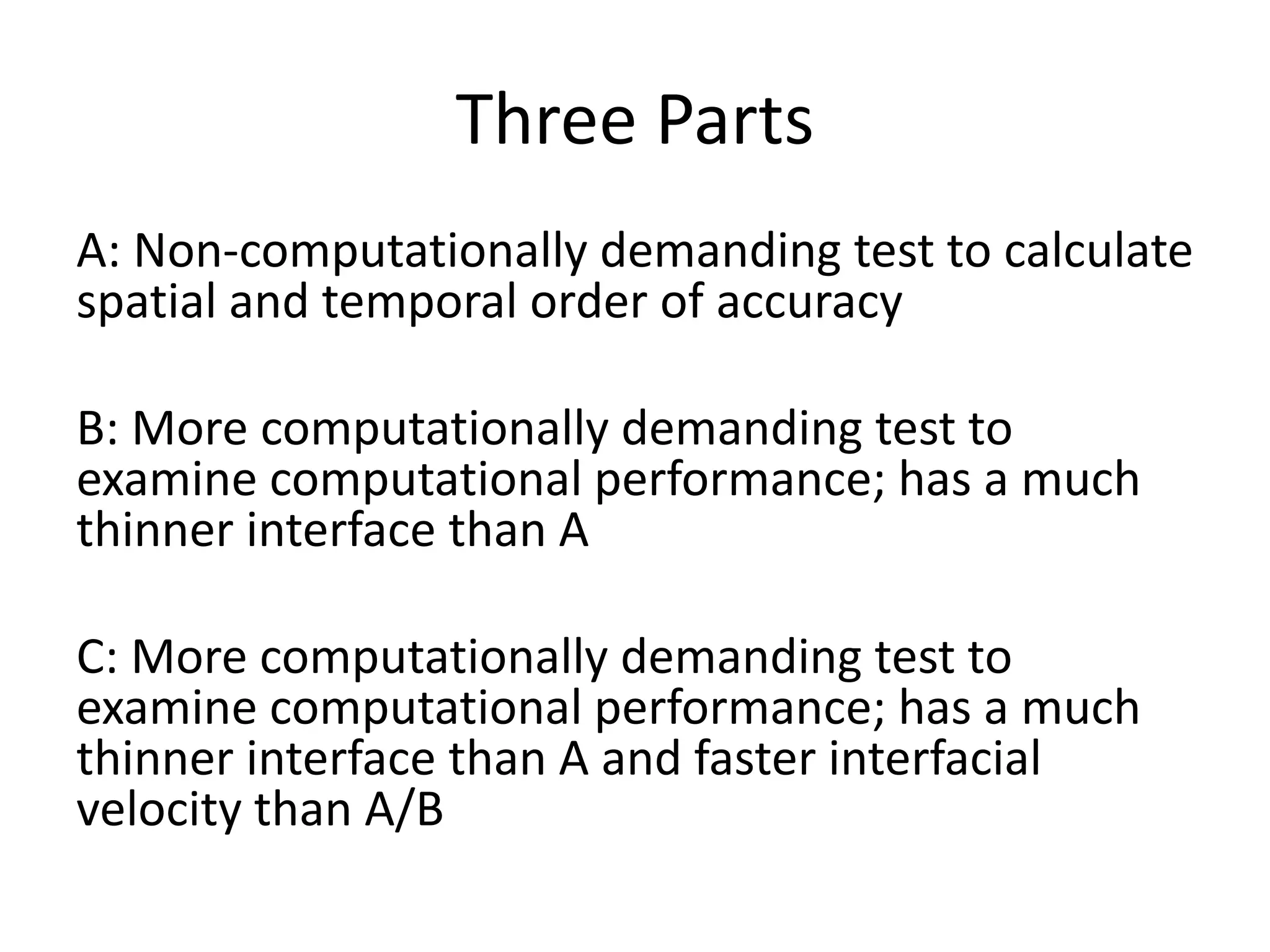
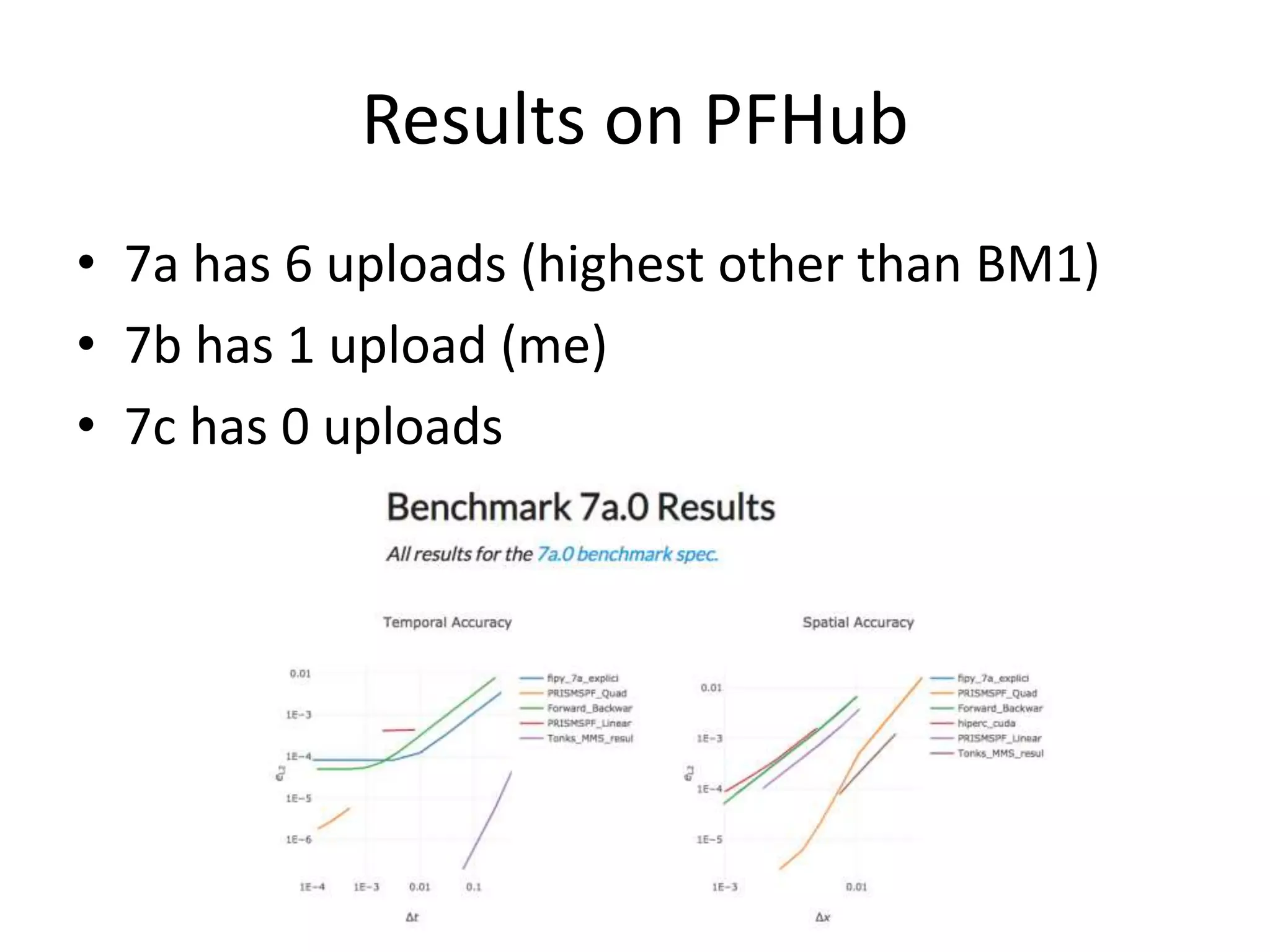
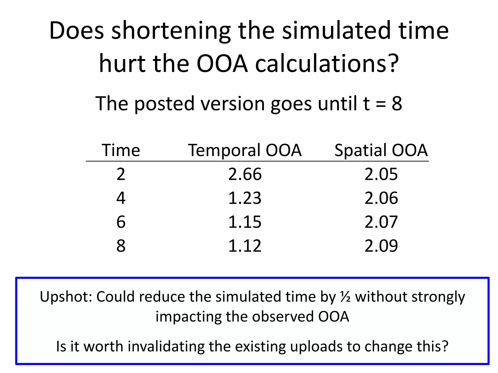
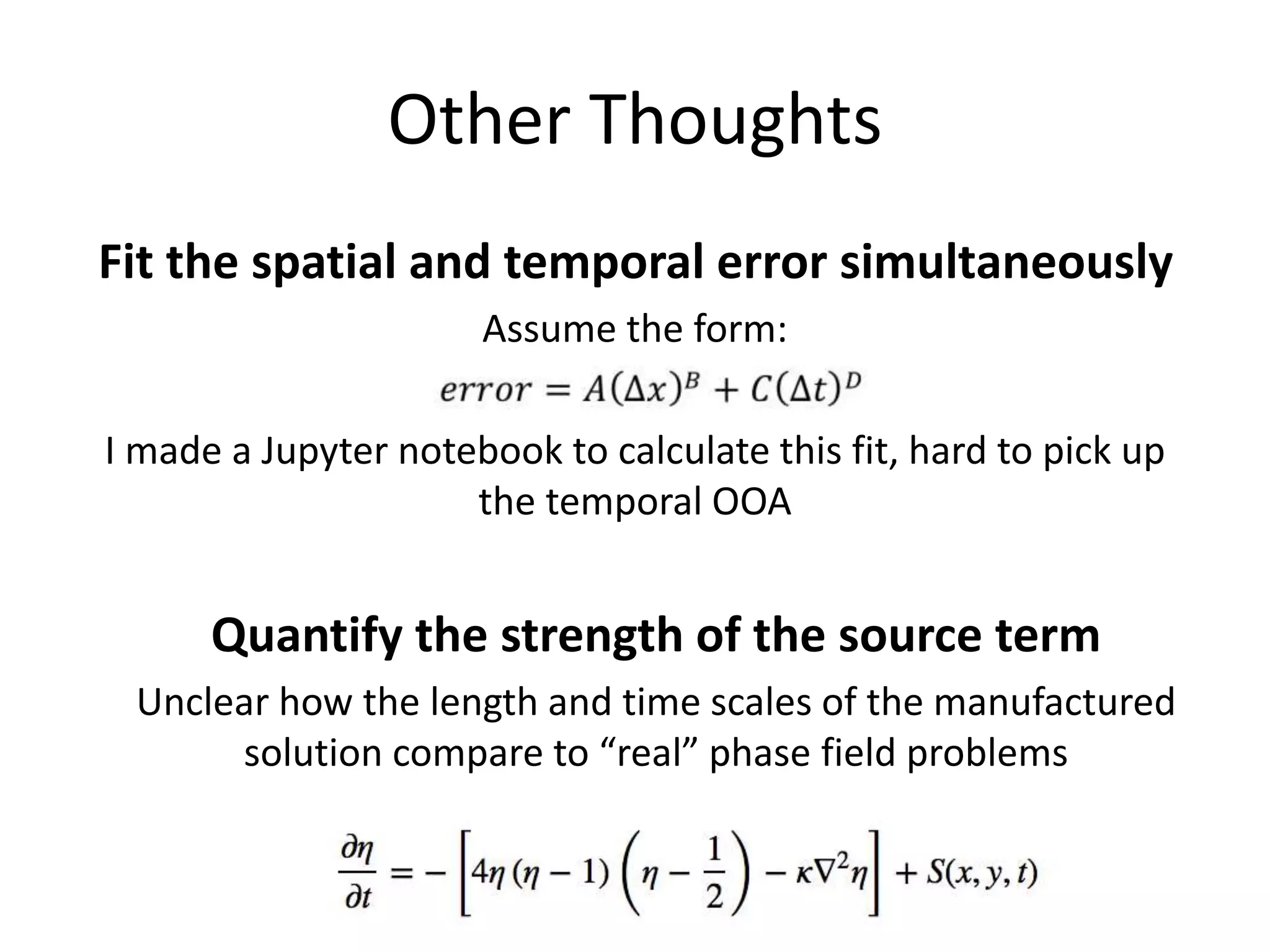
The document provides an update on Benchmark 7, which uses the Method of Manufactured Solutions (MMS) to test the order of accuracy of phase field codes. It has three primary objectives: 1) teach about MMS, 2) demonstrate code accuracy, and 3) enable code performance comparisons. Benchmark 7 consists of three parts with increasingly demanding tests involving thinner interfaces and faster velocities. Feedback from the last meeting included potentially removing Part C and shortening the simulation time to reduce runtimes. The author presents results showing the temporal order of accuracy could be calculated with half the simulation time without a large impact. Other discussion points include fitting the spatial and temporal errors simultaneously and quantifying the source term strength.

1. Update on Benchmark 7
Steve DeWitt
University of Michigan

2. Benchmark 7 Refresher
• Uses the Method of Manufactured Solutions
(MMS) for the Allen-Cahn equation
• Three Primary Objectives
1. Provide an example to teach phase field practitioners
about MMS
2. Have users demonstrate that their code achieves the
expected order of accuracy
3. Provide a platform for comparing the performance of
different codes (or options within a code) at known
error levels

3. The Manufactured Solution
For constant α, this is the
equilibrium solution to the
Allen-Cahn equation

4. Three Parts
A: Non-computationally demanding test to calculate
spatial and temporal order of accuracy
B: More computationally demanding test to
examine computational performance; has a much
thinner interface than A
C: More computationally demanding test to
examine computational performance; has a much
thinner interface than A and faster interfacial
velocity than A/B

5. Results on PFHub
• 7a has 6 uploads (highest other than BM1)
• 7b has 1 upload (me)
• 7c has 0 uploads

6. Feedback and Action Items from Last
Meeting
1. The run times can be long, especially for Parts B and C
1. Eliminate Part C as redundant; Part B is already taxing
enough
2. Consider reducing the length of the simulation (more
later)
2. The temporal order of accuracy is hard to get,
because spatial error dominates
1. Choose a simulation with a small time step to get a
baseline spatial error, subtract that off to get the nominal
temporal error
3. Fix the SymPy code
4. Tweak the order of the introduction
5. Clarify that OOA is not needed for Part B

7. Does shortening the simulated time
hurt the OOA calculations?
The posted version goes until t = 8
Time Temporal OOA Spatial OOA
2 2.66 2.05
4 1.23 2.06
6 1.15 2.07
8 1.12 2.09
Upshot: Could reduce the simulated time by ½ without strongly
impacting the observed OOA
Is it worth invalidating the existing uploads to change this?

8. Other Thoughts
Fit the spatial and temporal error simultaneously
Assume the form:
I made a Jupyter notebook to calculate this fit, hard to pick up
the temporal OOA
Quantify the strength of the source term
Unclear how the length and time scales of the manufactured
solution compare to “real” phase field problems