Fracture mechanics

Fracture mechanics
Nguyen Vinh Phu, PhD
nvinhphu@gmail.com
Researcher at Division of Computational Mechanics
Ton Duc Thang University
Program “Master of Science, Civil Engineering, Nguyen Vinh Phu 2012, Ton Duc Thang University”
1
Sunday, September 30, 1

Textbooks
• Anderson, T.L. (1995) Fracture Mechanics: Fundamentals
and Applications, 2nd Edition, CRC Press, USA.
• Gdoutos E.E (2005) Fracture Mechanics: an introduction,
2nd Edition, Springer.
• Zehnder, T.A. (2007) Lecture Notes on Fracture
Mechanics, Cornel University, Ithaca, New York
• imechanica.org
• wikipedia
2

Outline
• Brief recall on mechanics of materials
- stress/strain curves of metals, concrete
• Introduction
• Linear Elastic Fracture Mechanics (LEFM)
- Energy approach (Griffith, 1921, Orowan and Irwin 1948)
- Stress intensity factors (Irwin, 1960s)
• LEFM with small crack tip plasticity
- Irwin’s model (1960) and strip yield model
- Plastic zone size and shape
• Elastic-Plastic Fracture Mechanics
- Crack tip opening displacement (CTOD), Wells 1963
- J-integral (Rice, 1958)
• Mixed-mode crack propagation
3

Outline (cont.)
Fatigue
- Paris law
- Overload and crack retardation
Fracture of concrete
Computational fracture mechanics
- FEM, BEM, MMs
- XFEM
- cohesive crack model (Hillerborg, 1976)
- Continuum Damage Mechanics
- size effect (Bazant)
4

Stress-strain curves
Engineering stress and strain
0
0
Young’s modulus
ductile metals
strain hardening (tai ben)
Tension test
elastic unloading
!e =
P
A0
, ✏e =
#
L0
E !e = E✏e
5

Stress/strain curve
Wikipedia
fracture
necking=decrease of cross-sectional
area due to plastic deformation
1: ultimate tensile strength6

Stress-strain curves
True stress and true (logarithmic) strain:
(extension ratio)
!t =
P
A
, d✏t =
dL
L
! ✏t =
Z L
L0
1
L
dL = ln
L
L0
⌘
L
L0
Plastic deformation:volume does not change
dV = 0 ! AL = A0L0 !
L
L0
=
A
A0
Relationship between engineering and true stress/strain
!t = !e(1 + ✏e) = !e#
✏t = ln(1+✏e) = ln 7

Stress-strain curve
concrete
pre-peak post-peak(strain softening)
strain softening=increasing strain while stress decrease
8

Concrete
aggregates
cement paste
ITZ
fracture in concrete
9

Some common material
models
✏

no hardening
ys
✏
Linear elastic Elastic perfectly plastic
Will be used extensively in Fracture Mechanics
10

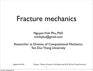
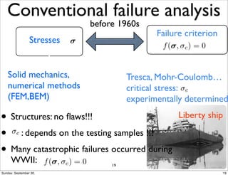
Strain energy density
Consider a linear elastic bar of stiffness k, length L, area A, subjected to a force F,
the work is
This work will be completely stored in the structure
in the form of strain energy. Therefore, the external work and strain
energy are equal to one another
In terms of stress/strain
F
u
W
x
✏x
u =
1
2
!x✏x
[J/m3]
u =
Z
!xd✏x
W =
Z u
0
Fdu =
Z u
0
kudu =
1
2
ku2 =
1
2
Fu
U = W =
1
2
Fu
U =
1
2
Fu =
1
2
F
A
u
L
AL
x
✏x
11

Plane problems
Kolosov coefficient
Poisson’s ratio
shear modulus
u =
1
2E
(!2x
+ !2
y + !2
z )
⌫
E
(!x!y + !y!z
+!z!x) +
1
2μ
(⌧ 2
xy + ⌧ 2
yz + ⌧ 2
zx)
 =
8
:
3 4⌫ plane strain
3 ⌫
plane stress
1 + ⌫
u =
1
4μ

 + 1
4
(2x
+ 2
y) 2(xy ⌧ 2
xy)

μ =
E
2(1 + ⌫)
12

Indicial notation
a 3D vector
+ xtwo times repeated index=sum,
summation/dummy index
!xx✏xx + !xy✏xy + !yx✏yx + !yy✏yy
@x
@23 x
i = 1, 2, 3
||x|| = pxixi
||x|| = pxkxk
!ij✏ij
ij,j = 0
i: free index (appears precisely once
in each side of an equation)
tensor notation
21
x = {x1, x2, q
x3}
||x|| =
x+ x22
+
@⌧xy
@y
= 0,
@y
@y
+
@⌧xy
@x
= 0
ijnj = ti
xxnx + xyny = tx
yxnx + yyny = ty
! : ✏
13

Engineering/matrix notation
!T✏ = !ij✏ij
x =
2
4
x1
x2
x3
3
5
Voigt notation
||x|| = xTx
=
2
4
xx
yy
xy
3
5 ✏ =
2
4
✏xx
✏yy
2✏xy
3
5
=

xx xy
xy yy

✏ =

✏xx ✏xy
✏xy ✏yy

||x|| = pxixi
!ij✏ij
14

Principal stresses
Principal direction
tan 2✓p =
Principal stresses are those stresses that act on principal surface. Principal
surface here means the surface where components of shear-stress is zero.
!1, !2 =
!xx + !yy
2 ±
s✓
!xx !yy
2
◆2
+ ⌧ 2
xy
2⌧xy
#xx #yy
15

Residual stresses
Residual stresses are stresses that remain
after the original cause of the stresses
(external forces, heat gradient) has been removed.
Wikipedia
Residual stresses always appear to some extent during
fabrication operations such as casting, rolling or welding.
Causes
• Heat treatment: welding, casting processes, cooling,
some parts contract more than others - residual
stresses
16

Residual stresses
TOTAL STRESS = APPLIED STRESS + RESIDUAL STRESS
Welding: produces tensile residual stresses - potential sites for cracks.
Knowledge of residual stresses is indispensable.
Measurement of residual stresses: FEM packages
17

Introduction
Cracks: ubiquitous !!!
18

Conventional failure analysis
Stresses
Failure criterion
Solid mechanics,
numerical methods
(FEM,BEM)
• Structures: no flaws!!!
• c
: depends on the testing samples !!!
• Many catastrophic failures occurred during
WWII:
Liberty ship
before 1960s
f(, c) = 0
f(, c) = 0
Tresca, Mohr-Coulomb…
critical stress:
c
experimentally determined

c
19

New Failure analysis
Stresses
f(, a,Kc) = 0
Flaw size a
Fracture
toughness
Fracture Mechanics (FM)
1970s
- FM plays a vital role in the design of every critical structural or machine
component in which durability and reliability are important issues (aircraft
components, nuclear pressure vessels, microelectronic devices).
- has also become a valuable tool for material scientists and engineers to guide
their efforts in developing materials with improved mechanical properties.
20

Design philosophies
• Safe life
The component is considered to be free of defects after
fabrication and is designed to remain defect-free during
service and withstand the maximum static or dynamic
working stresses for a certain period of time. If flaws, cracks,
or similar damages are visited during service, the component
should be discarded immediately.
• Damage tolerance
The component is designed to withstand the maximum static
or dynamic working stresses for a certain period of time
even in presence of flaws, cracks, or similar damages of
certain geometry and size.
21

Definitions
• Crack, Crack growth/propagation
• A fracture is the (local) separation of an
object or material into two, or more, pieces
under the action of stress.
• Fracture mechanics is the field of
mechanics concerned with the study of
the propagation of cracks in materials. It
uses methods of analytical solid mechanics
to calculate the driving force on a crack
and those of experimental solid mechanics
to characterize the material's resistance to
fracture (Wiki). 22

Objectives of FM
• What is the residual strength as a function of crack size?
• What is the critical crack size?
• How long does it take for a crack to grow from a certain
initial size to the critical size?
23

Brittle vs Ductile fracture
• In brittle fracture, no apparent plastic deformation takes place
before fracture, crack grows very fast!!!, usually strain is smaller
than 5%.
• In ductile fracture, extensive plastic deformation takes place
before fracture, crack propagates slowly (stable crack growth).
rough surfaces
Ductile fracture is preferable than brittle
failure!!! 24

Classification
Fracture mechanics:
• Linear Elastic Fracture Mechanics (LEFM)
- brittle-elastic materials: glass, concrete,
ice, ceramic etc.
• Elasto-Plastic Fracture Mechanics (EPFM)
- ductile materials: metals, polymer etc.
• Nonlinear Fracture Mechanics (NLFM)
25

Approaches to fracture
• Stress analysis
• Energy methods
• Computational fracture mechanics
• Micromechanisms of fracture (eg. atomic level)
• Experiments
• Applications of Fracture Mechanics
covered in
the course
26

Stress concentration
load lines
Geometry discontinuities: holes, corners, notches, cracks
etc: stress concentrators/risers
27

Stress concentration (cont.)
uniaxial
biaxial
28

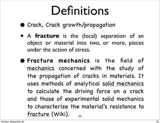
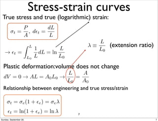
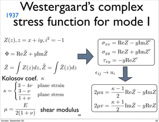
Elliptic hole
Inglis, 1913, theory of elasticity
3 =
✓
1 +
radius of curvature
⇢
2b
a
◆
1
⇢ =
b2
a
b
⇢
!
!1
!1 1
0 crack
!!!
!3 =
s
1 + 2
s
!3 = 2
b
⇢
stress concentration factor [-]
KT ⌘
3
1
= 1+
2b
a
29

Griffith’s work (brittle materials)
FM was developed during WWI by English aeronautical engineer A. A. Griffith to
explain the following observations:
• The stress needed to fracture bulk glass is around 100 MPa
• The theoretical stress needed for breaking atomic bonds is
approximately 10,000 MPa
• experiments on glass fibers that Griffith himself conducted: the
fracture stress increases as the fiber diameter decreases =
Hence the uniaxial tensile strength, which had been used
extensively to predict material failure before Griffith, could
not be a specimen-independent material property.
Griffith suggested that the low fracture strength observed in
experiments, as well as the size-dependence of strength, was due
to the presence of microscopic flaws in the bulk material.
30

Griffith’s size effect experiment
Size effect: ảnh hưởng kích thước
“the weakness of isotropic solids... is due to the presence of discontinuities or
flaws... The effective strength of technical materials could be increased 10 or
20 times at least if these flaws could be eliminated.''
31

Griffith’s experiment
• Glass fibers with artificial cracks (much larger
than natural crack-like flaws), tension tests
c =
const
pa
Energy approach
s
!3 = 2
b
⇢
!1
cpa = const
32

Energy balance during
crack growth
external work
kinetic energy
surface energy
= ˙U
e + ˙Up + ˙U
k + ˙U

internal strain energy
˙W
All changes with respect to time are caused by changes in
crack size:
@(·)
@t
Energy equation is rewritten:
slow process
@W
@a
=
@Ue
@a
=
+
@(·)
@a
@Up
@a
@a
@t
+
@U
@a
It indicates that the work rate supplied to the continuum by the applied loads is equal
to the rate of the elastic strain energy and plastic strain work plus the energy
dissipated in crack propagation
33

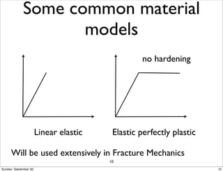
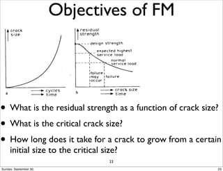
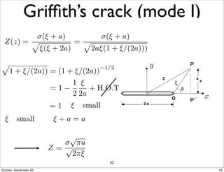
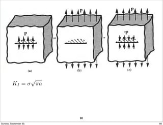
Potential energy
Brittle materials: no plastic deformation
γs is energy required to form a unit of new surface
(two new material surfaces)
Inglis’ solution
(plane stress, constant load)
Griffith’s through-thickness crack
[J/m2=N/m]
⇧ = Ue W
@⇧
@Up

=
+
@a
@a
@U
@a

@⇧
@a
=
@U
@a

@⇧
@a
= 2s

@⇧
@a
=
⇡#2a
E
⇡2a
E
= 2#s ! c =
r
2E#s
⇡a
!cpa =
✓
2Es
⇡
◆1/2
34

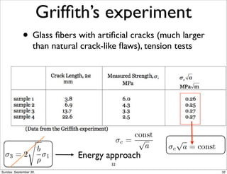
[N/m2]
⇡2a
E
= 2#s ! c =
r
2E#s
⇡a
⇡2a
E
= 2#s ! c =
r
2E#s
⇡a
E : MPa=N/m2
s : N/m
a: m
check dimension
Dimensional Analysis
App. of B = 1
dimensional analysis
u =
1
2
!✏ =
1
2
!2
E U = !
2
E
a2
[N/m2]
35

[N/m2]
⇡2a
E
= 2#s ! c =
r
2E#s
⇡a
⇡2a
E
= 2#s ! c =
r
2E#s
⇡a
E : MPa=N/m2
s : N/m
a: m
check dimension
Dimensional Analysis
! = ⇡ B = 1 App. of
dimensional analysis
u =
1
2
!✏ =
1
2
!2
E U = !
2
E
a2
[N/m2]
35

Energy equation for
ductile materials Plane stress
!c =
r
2Es
⇡a
Griffith (1921), ideally brittle solids
Irwin, Orowan (1948), metals
plastic work per unit area of surface created
(metals)
Griffith’s work was ignored for almost 20 years
!c =
r
2Es
⇡a
!c =
r
2E(s + p)
⇡a
p
p s
p ⇡ 103s
36

Energy release rate
d⇧
dA
Irwin 1956
G ⌘ −
G: energy released during fracture per unit of newly
created fracture surface area
the resistance of the material
that must be overcome for
crack growth
G = |2 {+z p}
energy available for crack growth (crack driving force)
Energy release rate failure criterion
Gc
G Gc
fracture energy, considered to be a material property (independent of the
applied loads and the geometry of the body).
37

Energy release rate
d⇧
dA
Irwin 1956
G ⌘ −
Griffith
G: energy released during fracture per unit of newly
created fracture surface area
the resistance of the material
that must be overcome for
crack growth
G = |2 {+z p}
energy available for crack growth (crack driving force)
Energy release rate failure criterion
Gc
G Gc
fracture energy, considered to be a material property (independent of the
applied loads and the geometry of the body).
37

G from experiment
G ⌘ −
d⇧
dA
a1: OA, triangle OAC=U
Fixed grips Dead loads
G =
1
B
(OAB)
a
G =
1
B
(OAB)
a
⇧ = Ue W
W = 0 ! Ue 0
B: thickness
elastic strain energy stored in the body is decreasing—is
being released
a2: OB, triangle OBC=U
OAB=ABCD-(OBD-OAC)
38

G from experiments
G =
1
B
shaded area
a4 a3 39

Crack extension resistance
curve (R-curve)
G =
d⇧
dA
=
dU
dA
+
dUp
dA
G = R
R ⌘
dU
dA
+
dUp
dA
R-curve
Resistance to fracture increases with growing
crack size in elastic-plastic materials.
R = R(a) Irwin
crack driving
force curve
SLOW
Irwin
Stable crack growth: fracture
resistance of thin specimens
is represented by a curve not
a single parameter.
40

R-curve shapes
flat R-curve
(ideally brittle materials)
rising R-curve
(ductile metals)
G = R,
dG
da 
dR
da
stable crack growth
crack grows then stops,
only grows further if
there is an increase of
applied load
G =
⇡2a
E
slope
41

G in terms of compliance
Fixed grips
inverse of stiffness
P
K u
C
C =
u
P
dUe = Ue(a + da) Ue(a)
=
1
2
(P + dP)u
1
2
Pu
=
1
2
dPu
G =
1
2B
u
dP
da
G =
1
2B
u2
C2
dC
da
=
1
2B
P2 dC
da
a
a + da
u
P
dP
dA = Bda
G =
dW dUe
42 dA

inverse of stiffness
Fixed load
G =
1
2B
P2 dC
da
P
K u
C
C =
u
P
dUe =
1
2
P(u + du)
1
2
Pu
=
1
2
Pdu
dW = Pdu
G =
1
2B
P
du
da
P a + da
a
u
du
G =
dW dUe
43 dA

G =
Fixed grips Fixed loads
1
2B
u2
C2
dC
da
=
1
2B
P2 dC
da
G =
1
2B
P2 dC
da
Strain energy release rate is identical for fixed grips and
fixed loads.
Strain energy release rate is proportional to the
differentiation of the compliance with respect to the crack
length.
44

Stress analysis of
isotropic linear elastic
cracked solids
45

Airy stress function for
solving 2D linear elasticity problems
@x
@x
+
@⌧xy
@y
= 0,
@y
@y
+
@⌧xy
@x
Equilibrium: = 0
Airy stress
function :
Compatibility
condition:
Bi-harmonic equation
!x =
@2
@y2 , !y =
@2
@x2 , ⌧xy =
@2
@x@y
r4 =
@4
@x4 + 2
@4
@x2@y2 +
@4
@y4 = 0
For a given problem, choose an appropriate
that
satisfies (*) and the boundary conditions.
! !ij ! ✏ij ! ui

(*)
46

Crack modes
ar
47

Crack modes
48

Westergaard’s complex
stress function for mode I 1937
shear modulus
Kolosov coef.
μ =
E
2(1 + ⌫)
xx = ReZ yImZ0
yy = ReZ + yImZ0
⌧xy = yReZ0
✏ij ! ui
 =
8
:
3 4⌫ plane strain
3 ⌫
1 + ⌫
plane stress 2μu =
 1
2
Re ¯ Z yImZ
2μv =
 + 1
2
Im ¯ Z yReZ
Z(z), z = x + iy, i2 = 1
= Re¯¯
Z + yIm ¯ Z
¯ Z =
Z
Z(z)dz, ¯¯
Z =
Z
¯ Z(z)dz

49

Griffith’s crack (mode I)
y = 0, |x| a
Z(z) =
p!(⇠ + a)
⇠(⇠ + 2a)
boundary conditions
⇠ = z a, ⇠ = rei✓
Z =
!p⇡a
p2⇡⇠
infinite plate
Z(z) =
z
pz2 − a2
(x, y)!1: !xx = !yy = !, ⌧xy = 0
|x| a,y = 0 : !yy = ⌧xy = 0
Z(z) =
x
px2 − a2
is imaginary
Z(z) =
p
1 (a/z)2
(x, y)!1: z !1 Z !
1I
I
Z0(z) = −
a2
(z2 − a2)3/2 ! 0
50
xx = ReZ yImZ0
yy = ReZ + yImZ0
⌧xy = yReZ0

Z(z) =
Z(z) =
z
pz2 − a2
p!(⇠ + a)
⇠(⇠ + 2a)
(x, y)!1: !xx = !yy = !, ⌧xy = 0
|x| a,y = 0 : !yy = ⌧xy = 0
boundary conditions
x
y
⇠ = z a, ⇠ = rei✓
Z =
!p⇡a
p2⇡⇠
infinite plate 51

(x, y)!1: !xx = !yy = !, ⌧xy = 0
|x| a,y = 0 : !yy = ⌧xy = 0
x
y
⇠ small
Z =
!p⇡a
p2⇡⇠
⇠ small
Z =
!p⇡a
p2⇡⇠
Z(z) =
p!(⇠ + a)
⇠(⇠ + 2a)
=
p !(⇠ + a)
2a⇠(1 + ⇠/(2a)))
p
1 + ⇠/(2a)) = (1 + ⇠/(2a))1/2
= 1
1
2
⇠
2a
+ H.O.T
= 1
⇠ small ⇠ + a = a
52

Recall
xx = ReZ yImZ0
yy = ReZ + yImZ0
⌧xy = yReZ0
eix = cos x i sin x
y = r sin ✓
sin ✓ = 2sin
✓
2
cos
✓
2
Crack tip stress field
inverse square root
Z(z) =
KI p2⇡⇠
,KI = #p⇡a
Z(z) =
KI p2⇡r
ei✓/2
Z0(z) = −
1
2
KI p2⇡
⇠−3/2 = −
KI
2rp2⇡r
e−i3✓/2
⇠ = rei✓
!xx =
KI p2⇡r
cos
✓
2
✓
1 − sin
✓
2
cos
3✓
2
◆
!yy =
KI p2⇡r
cos
✓
2
✓
1 + sin
✓
2
cos
3✓
2
◆
⌧xy =
KI p2⇡r
sin
✓
2
cos
✓
2
sin
3✓
2
53 r ! 0 : ij ! 1

Recall
xx = ReZ yImZ0
yy = ReZ + yImZ0
⌧xy = yReZ0
eix = cos x i sin x
y = r sin ✓
sin ✓ = 2sin
1
pr
✓
2
cos
singularity
✓
2
Crack tip stress field
inverse square root
Z(z) =
KI p2⇡⇠
,KI = #p⇡a
Z(z) =
KI p2⇡r
ei✓/2
Z0(z) = −
1
2
KI p2⇡
⇠−3/2 = −
KI
2rp2⇡r
e−i3✓/2
⇠ = rei✓
!xx =
KI p2⇡r
cos
✓
2
✓
1 − sin
✓
2
cos
3✓
2
◆
!yy =
KI p2⇡r
cos
✓
2
✓
1 + sin
✓
2
cos
3✓
2
◆
⌧xy =
KI p2⇡r
sin
✓
2
cos
✓
2
sin
3✓
2
53 r ! 0 : ij ! 1

Plane strain problems
Hooke’s law
Plane strain
!z = ⌫(!x + !y)
!z = 2⌫
KI
2⇡r
cos
✓
2
✏zz =
1
E
(⌫#xx ⌫#yy + #zz)
✏zz = 0
!xx =
KI p2⇡r
cos
✓
2
✓
1 − sin
✓
2
cos
3✓
2
◆
!yy =
KI p2⇡r
cos
✓
2
✓
1 + sin
✓
2
cos
3✓
2
◆
⌧xy =
KI p2⇡r
sin
✓
2
cos
✓
2
sin
3✓
2
54

Stresses on the crack plane
On the crack plane
✓ = 0, r = x
!xx = !yy =
KI p2⇡x
⌧xy = 0
crack plane is a principal plane
with the following principal
stresses
1 = 2 = xx = yy
!xx =
KI p2⇡r
cos
✓
2
✓
1 − sin
✓
2
cos
3✓
2
◆
!yy =
KI p2⇡r
cos
✓
2
✓
1 + sin
✓
2
cos
3✓
2
◆
⌧xy =
KI p2⇡r
sin
✓
2
cos
✓
2
sin
3✓
2
55

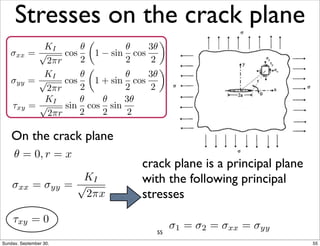
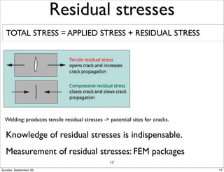
Stress Intensity Factor (SIF)
KI
• Stresses-K: linearly proportional
• K uniquely defines the crack tip stress field
• modes I, II and III:
KI,KII,KIII
• LEFM: single-parameter
SIMILITUDE
!xx =
KI p2⇡r
cos
✓
2
✓
1 − sin
✓
2
cos
3✓
2
◆
!yy =
KI p2⇡r
cos
✓
2
✓
1 + sin
✓
2
cos
3✓
2
◆
⌧xy =
KI p2⇡r
sin
✓
2
cos
✓
2
sin
3✓
2
KI = !p⇡a
[MPapm]
56

Singular dominated zone
1
1
crack tip
K-dominated zone
!yy =
KI p2⇡r
cos
✓
2
✓
1 + sin
✓
2
cos
3✓
2
◆
(crack plane)
!xx =
KI p2⇡r
cos
✓
2
✓
1 − sin
✓
2
cos
3✓
2
◆
!yy =
KI p2⇡r
cos
✓
2
✓
1 + sin
✓
2
cos
3✓
2
◆
⌧xy =
KI p2⇡r
sin
✓
2
cos
✓
2
sin
3✓
2 57

Mode I: displacement field
Displacement field
Recall
2μu =
 1
2
Re ¯ Z yImZ
2μv =
 + 1
2
Im ¯ Z yReZ
Z(z) =
KI p2⇡r
✓
cos
✓
2 − i sin
✓
2
◆
Z(z) =
KI p2⇡⇠
¯ Z =
Z
Z(z)dz
¯ Z(z) = 2
KI p2⇡
⇠1/2 = 2KI
r
r
2⇡
✓
cos
✓
2
+ i sin
✓
2
◆
u =
KI
2μ
r
r
2⇡
cos
✓
2
✓
 1 + 2sin2 ✓
2
◆
v =
KI
2μ
r
r
2⇡
sin
✓
2
✓
 + 1 2 cos2 ✓
2
◆
z = ⇠ + a
⇠ = rei✓
eix = cos x i sin x
58

Crack face displacement
2μv =
 + 1
2
y = 0,−a  x  a
Im ¯ Z yReZ
Z(z) =
x
px2 − a2
¯ Z(z) =
p
x2 a2
v =
 + 1
4μ
Im ¯ Z
¯ Z(z) = i(
p
a2 x2)
−a  x  a i = p−1
v =
 + 1
4μ

p
a2 x2
Crack Opening Displacement
COD = 2v =
 + 1
2μ

p
a2 x2
ellipse
59

Crack tip stress field in
polar coordinates-mode I
stress transformation
!ij =
KI p⇡a
fij(✓)
!rr =
KI p2⇡r
✓
5
4
cos
✓
2 −
1
4
cos
3✓
2
◆
!✓✓ =
KI p2⇡r
✓
3
4
cos
✓
2
+
1
4
cos
3✓
2
◆
⌧r✓ =
KI p2⇡r
✓
1
4
sin
✓
2
+
1
4
sin
3✓
2
◆
60

Principal crack tip stresses
!1, !2 =
!xx + !yy
2 ±
s✓
!xx !yy
2
◆2
+ ⌧ 2
xy
!1 =
KI p2⇡r
cos
✓
2
✓
1 + sin
✓
2
◆
!2 =
KI p2⇡r
cos
✓
2
✓
1 − sin
✓
2
◆
!3 =
8
:
0 plane stress
2⌫KI ✓
p2⇡cos
r
2
!xx =
KI p2⇡r
cos
✓
2
✓
1 − sin
✓
2
cos
3✓
2
◆
!yy =
KI p2⇡r
cos
✓
2
✓
1 + sin
✓
2
cos
3✓
2
◆
⌧xy =
KI p2⇡r
sin
✓
2
cos
✓
2
sin
3✓
2
plane strain !3 = ⌫(!1 + !2)
61

Mode II problem
Boundary conditions
Stress function
(x, y)!1: !xx = !yy = 0, ⌧xy = ⌧
|x| a,y = 0 : !yy = ⌧xy = 0
Z = −
i⌧z
pz2 − a2
xx = ReZ yImZ0
yy = ReZ + yImZ0
⌧xy = yReZ0
Check BCs
62

Mode II problem
Boundary conditions
Stress function
mode II SIF
(x, y)!1: !xx = !yy = 0, ⌧xy = ⌧
|x| a,y = 0 : !yy = ⌧xy = 0
KII = ⌧p⇡a
Z = −
i⌧z
pz2 − a2
!xx = −
KII p2⇡r
sin
✓
2
✓
2 + cos
✓
2
cos
3✓
2
◆
!yy =
KII p2⇡r
sin
✓
2
cos
✓
2
cos
3✓
2
⌧xy =
KII p2⇡r
cos
✓
2
✓
1 − sin
✓
2
sin
3✓
2
◆
63

Mode II problem (cont.)
(x, Z y)!= −
1: !xx = !yy = 0, ⌧xy = ⌧
|x| a,y = 0 : !yy = ⌧xy = 0
i⌧z
pz2 − a2
Stress function
(x, y)!1: !xx = !yy = 0, ⌧xy = ⌧
|x| a,y = 0 : !yy = ⌧xy = 0
mode II SIF
Z = −
i⌧z
pz2 − a2
KII = ⌧p⇡a
u =
KII
2μ
r
r
2⇡
sin
✓
2
✓
 + 1 + 2 cos2 ✓
2
◆
v =
KII
2μ
r
r
2⇡
cos
✓
2
✓
 1 2 sin2 ✓
2
◆
64

Mode III problem
65

Universal nature of the
asymptotic stress field
Westergaards, Sneddon etc.
KI p2⇡r
(mode I) (mode II)
!ij =
K
p2⇡r
fij(✓) + H.O.T
!xx =
Irwin
cos
✓
2
✓
1 − sin
✓
2
cos
3✓
2
◆
!yy =
KI p2⇡r
cos
✓
2
✓
1 + sin
✓
2
cos
3✓
2
◆
⌧xy =
KI p2⇡r
sin
✓
2
cos
✓
2
sin
3✓
2
!xx = −
KII p2⇡r
sin
✓
2
✓
2 + cos
✓
2
cos
3✓
2
◆
!yy =
KII p2⇡r
sin
✓
2
cos
✓
2
cos
3✓
2
⌧xy =
KII p2⇡r
cos
✓
2
✓
1 − sin
✓
2
sin
3✓
2
◆
66

Inclined crack in tension
!1 = !x cos2 ✓ + 2 sin ✓ cos ✓⌧xy + sin2 ✓!y
!2 = !y cos2 ✓ 2 sin✓ cos ✓⌧xy + sin2 ✓!x
⌧12 = x cos ✓ sin ✓ + cos 2✓⌧xy + 0.5 sin2✓y
!1 = (sin2 )!
!2 = (cos2 )!
⌧12 = (sin cos )#
Recall
KI = !yp⇡a
KII = ⌧xyp⇡a
KI = !p⇡a cos2 #
KII = !p⇡a sin # cos #
+
Final result
67

Inclined crack in tension
!1 = !x cos2 ✓ + 2 sin ✓ cos ✓⌧xy + sin2 ✓!y
!2 = !y cos2 ✓ 2 sin✓ cos ✓⌧xy + sin2 ✓!x
⌧12 = x cos ✓ sin ✓ + cos 2✓⌧xy + 0.5 sin2✓y
!1 = (sin2 )!
!2 = (cos2 )!
⌧12 = (sin cos )#
Recall
KI = !yp⇡a
KII = ⌧xyp⇡a
KI = !p⇡a cos2 #
KII = !p⇡a sin # cos #
+
Final result
2 1
67

Cylindrical pressure vessel with an inclined
through-thickness crack
z =
pR
2t
✓ =
pR
t
R
t 10 thin-walled pressure
KI =
(⇡R2)p = (2⇡Rt)z
(l2R)p = (2lt)✓
pR
2t
p⇡a(1 + sin2 )
KII =
pR
2t
p⇡a sin cos
closed-ends
68

Cylindrical pressure vessel with an inclined
through-thickness crack
z =
pR
2t
✓ =
pR
t
KI =
This is why an overcooked hotdog usually
cracks along the longitudinal direction first
(i.e. its skin fails from hoop stress, generated
by internal steam pressure).
pR
2t
✓ = 2z
p⇡a(1 + sin2 )
KII =
pR
2t
p⇡a sin cos
?
Equilibrium
69

Computation of SIFs
• Analytical methods (limitation: simple geometry)
- superposition methods
- weight/Green functions
• Numerical methods (FEM, BEM, XFEM)
numerical solutions - data fit - SIF
handbooks
• Experimental methods
- photoelasticity
70

SIF for finite size samples
Exact (closed-form) solution for SIFs: simple crack
geometries in an infinite plate.
Cracks in finite plate: influence of external boundaries
cannot be neglected - generally, no exact solution
71

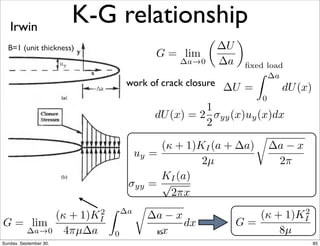
SIF for finite size samples
KI KI
force lines are compressed-
higher stress concentration
geometry/correction
factor [-]
dimensional
analysis
KI = f(a/W)!p⇡a a ⌧ W : f(a/W) ⇡ 1
72

SIFs handbook
73

SIFs handbook
74

SIFs handbook
75

Reference stress
KI = !p⇡a
KI = !maxmaxp⇡a
KI = !xaxap⇡a
!xa = !max
max
xa
=
!max
1 2a/W
Non-uniform stress distribution

for which reference stress!!!
76

Reference stress
KI = !p⇡a
KI = !maxmaxp⇡a
KI = !xaxap⇡a
!xa = !max
max
xa
=
!max
1 2a/W
chosen
Non-uniform stress distribution

for which reference stress!!!
76

Superposition method
A sample in mode I subjected to tension and bending:
!ij =
Ktension
Ip
2⇡r
fij(✓) +
Kbending
Ip
2⇡r
fij(✓)
!ij =
I + Kbending
Ktension
I p2⇡r
fij(✓)
I + Kbending
KI = Ktension
I
Is superposition of SIFs of different crack modes
possible?
77

Determine the stress intensity factor for an edge cracked
plate subjected to a combined tension and bending.
Kbend
I = fM(a/W)
6M
BW2
p⇡a Kten
I = fP (a/W)
P
BW
p⇡a
a/W = 0.2
1.055 1.12
KI =
✓
1.055
6M
BW2 + 1.12
P
BW
◆
p⇡a
B thickness
Solution
78

Superposition method
Centered crack under internal pressure
KId + KIe = KIb = 0 ! KIe = −KId = −!p⇡a
This result is useful for surface flaws along the
internal wall of pressure vessels.
79

KI = !p⇡a
80

SIFs: asymmetric loadings
Procedure: build up the case from symmetric
cases and then to subtract the superfluous
loadings.
KA = KB + KC KD
KA = (KB + KC)/2
81

Two small cracks at a hole
a
3 edge crack hole as a part of the crack
82

Photoelasticity
Wikipedia
Photoelasticity is an experimental method to determine the stress distribution in a material.
The method is mostly used in cases where mathematical methods become quite cumbersome.
Unlike the analytical methods of stress determination, photoelasticity gives a fairly accurate
picture of stress distribution, even around abrupt discontinuities in a material. The method is an
important tool for determining critical stress points in a material, and is used for determining
stress concentration in irregular geometries.
83

K-G relationship
So far, two parameters that describe the
behavior of cracks: K and G.
K: local behavior (tip stresses)
G: global behavior (energy)
Irwin: for linear elastic materials, these two params are
uniquely related
Crack closure analysis: work
to open the crack = work to close
the crack
84

K-G relationship Irwin
dU(x)
✓ = ⇡
work of crack closure
U =
✓ = 0
B=1 (unit thickness)
KI (a)
G = lim
a!0
( + 1)K2
I
4⇡μa
Z a
0
r
dU(x) = 2
a x
x
dx G =
Z a
0
( + 1)K2
I
8μ
uy =
( + 1)KI (a + a)
2μ
r
a x
2⇡
!yy =
KI (a)
p2⇡x
1
2
yy(x)uy(x)dx
G = lim
a!0
✓
U
a
◆
fixed load
85

K-G relationship (cont.)
Mode I
Mixed mode
GI =
8
:
K2
I
E
plane stress
(1 v2)
K2
I
E
plane strain
G =
K2
I
E0
+
K2
II
E0
+
K2
III
2μ
• Equivalence of the strain energy release rate and SIF approach
• Mixed mode: G is scalar = mode contributions are additive
• Assumption: self-similar crack growth!!!
Self-similar crack growth: planar crack remains planar ( da
same
direction as )
a 86

SIF in terms of compliance
1
2B
P2 dC
G = B: thickness
da
GI =
K2
I
E0
K2
I =
E0P2
2B
dC
da
A series of specimens with different crack lengths: measure the
compliance C for each specimen - dC/da - K and G
87

Units
88

Example
89

G =
1
2B
OAiAj
aj ai
Gc for different crack lengths are almost the same: flat R-curve.
90

Examples
Double cantilever beam (DCB)
a increases - G increase
G =
1
2B
P2 dC
da
load control
G =
1
2B
u2
C2
dC
da
disp. control
load control
G =
3u2Eh3
16a4
a increases - G decreases!!!
93

Compliance-SIF
K =
r
sec
⇡a
W
p⇡a
G =
P2
2
dC
dA
=
P2
4B
dC
da
K2
E
P2
4B
G =
dC
da
=
sec ⇡a
W !2⇡a
E
dC
da
=
sec ⇡a
W !2⇡a4B
P2E
dC
da
=
4
EBW2 ⇡a sec
⇡a
W
C =
Z a
0
4
EBW2 ⇡a sec
⇡a
W
da + C0
C =
4
EB⇡
ln
⇣
cos
⇡a
W
⌘
+
H
EBW
C0 =

P
=
H
EBW
H
94

C/C0 =
4
⇡
W
H
ln
⇣
cos
⇡a
W
⌘
+ 1
compliance rapidly increases
95

K as a failure criterion
Failure criterion
fracture toughness
W,Kc • Problem 1: given crack length a, compute the
maximum allowable applied stress
• Problem 2: for a specific applied stress, compute the

maximum permissible crack length (critical crack
length)
ac
• Problem 3: compute provided crack length and
stress at fracture
K = Kc f(a/W)!p⇡a = Kc
!max =
Kc
f(a/W)p⇡a
f(ac/W)!p⇡ac = Kc
Kc
! ac
Kc = f(ac/W)!p⇡ac
96

Example
97

Example solution
z =
pR
2t
✓ =
pR
t
a
KI = 1.12!✓p⇡a
KI = KIc/S
problem 1 problem 2
p = 12MPa
a = 1mm
98

Example
Griffith Irwin
!c =
r
2Es
⇡a
=5.8 Mpa !c =
KIc p⇡a =479 Mpa
99

Mixed-mode fracture
KI = KIc
KII = KIIc
KIII = KIIIc
KIc KIIc,KIIIc
Superposition cannot be applied to SIF.
However, energy can.
G =
K2
I
E0
+
K2
II
E0
Gc =
K2
Ic
E0
lowest Kc: safe
Fracture occurs when
G = Gc
K2
I + K2
II = K2
Ic
100

Experiment verification of the
mixed-mode failure criterion
K2
I + K2
II = K2
Ic
Data points do not fall exactly on the circle.
a circle in
KI, KII plane
G =
( + 1)K2
I
8μ self-similar growth
✓
KI
KIc
◆2
+
✓
KII
KIIc
◆2
= 1
101

G: crack driving force - crack will grow in the
direction that G is maximum
102

Crack tip plasticity
• Irwin’s model
• Strip Yield model
• Plane stress vs plane strain
• Plastic zone shape
103

Introduction
• Griffith's theory provides excellent agreement with experimental data for
brittle materials such as glass. For ductile materials such as steel, the surface
energy (γ) predicted by Griffith's theory is usually unrealistically high. A
group working under G. R. Irwin at the U.S. Naval Research Laboratory
(NRL) during World War II realized that plasticity must play a significant role
in the fracture of ductile materials.
crack tip
(SSY)
Small-scale yielding:
LEFM still applies with
minor modifications done
by G. R. Irwin
R ⌧ D
104

Validity of K in presence of a
plastic zone
crack tip Fracture process usually occurs in
the inelastic region not the K-dominant
zone.
is SIF a valid failure criterion for materials that
exhibit inelastic deformation at the tip ?
105

Validity of K in presence of
a plastic zone
same K-same stresses applied on the disk
stress fields in the plastic zone: the same
K still uniquely characterizes the crack tip
conditions in the presence of a small
plastic zone.
[Anderson]
LEFM solution
106

Paradox of a sharp crack
At crack tip:
r = 0 ! ij = 1
An infinitely sharp crack is merely a mathematical
abstraction.
Crack tip stresses are finite because (i) crack tip
radius is finite (materials are made of atoms) and (ii)
plastic deformation makes the crack blunt.
107

Plastic correction
• A cracked body in a plane stress condition
• Material: elastic perfectly plastic with yield stress
On the crack plane
stress singularity is truncated by
yielding at crack tip
ys
KI p2⇡r
✓ = 0
(yield occurs)
!yy =
yy = ys
r1 =
K2
I
2⇡2
ys
first order approximation of plastic zone size: equilibrium
is not satisfied
ys
108

Irwin’s plastic correction
109

plate behaves as with a longer crack
stress redistribution: yellow
area=hatched area
Plane strain
plastic zone: a CIRCLE !!!
rp = 2r1 =
K2
I
⇡2
ys
rp =
1
3⇡
K2
I
2
ys 110
ysr1 =
Z r1
0
yydr

Plane stress Plane strain
1 = 2 = yy, 3 = 0 1 = 2 = yy
!3 = ⌫(!xx + !yy) = 2⌫!yy
3 = 0.66yy ⌫ = 0.33
1 3 = ys
Tresca’s criterion
1 = ys
y = ys y = 3ys
111

ysr1 =
Z r1
0
yydr
LEFM:
rp =
1
3⇡
K2
I
2
ys
crack tip
R ⌧ D
rp is small
ys is big and KIc is small
LEFM is better applicable to materials of high yield
strength and low fracture toughness
112

Plastic zone shape
von-Mises criterion
e =
1
p2
!
(1 − 2)2 + (1 − 3)2 + (2 − 3)21/2
Mode I, principal stresses
e = ys
!1 =
KI p2⇡r
cos
✓
2
✓
1 + sin
✓
2
◆
!2 =
KI p2⇡r
cos
✓
2
✓
1 − sin
✓
2
◆
!3 =
8
:
0 plane stress
2⌫KI ✓
p2⇡cos
r
2
plane strain
ry(✓) =
1
4⇡
✓
KI
#ys
◆2 
1 + cos ✓ +
3
2
sin2 ✓
$
ry(✓) =
1
4⇡
✓
KI
#ys
◆2 
(1 2μ)2(1 + cos ✓) +
3
2
plane stress
sin2 ✓
$
113

Plastic zone shape
plastic zone shape (mode I, von-Mises criterion)
ry(✓) =
1
4⇡
✓
KI
#ys
◆2 
1 + cos ✓ +
3
2
sin2 ✓
$
0.6
0.4
0.2
0
−0.2
−0.4
−0.6−0.4−0.2 0 0.2 0.4 0.6 0.8
114
−0.6
r
p
/(K
/(/ my
I
))2
))2
/(/ my
I
/(K
r
p
plane stress
plane strain

Plane stress/plane strain
dog-bone shape
constrained by the
surrounding material
• Plane stress failure: in general, ductile
• Plane strain failure: in general, brittle
115

Plane stress/plane strain
toughness depends on thickness
Plane strain fracture toughness
lowest K (safe)
KIc
(Irwin)
116
Kc = KIc
1 +
1.4
B2

KIc
ys
#4
!1/2

Fracture toughness tests
• Prediction of failure in real-world applications: need
the value of fracture toughness
• Tests on cracked samples: PLANE STRAIN condition!!!
Compact Tension Test
ASTM (based on
Irwin’s model)
Constraint
conditions
KI =
P
BpW
⇣
2 +
a
W
⌘ 
0.886 + 4.64
a
W − 13.32
⇣ a
W
⌘2
+ 14.72(
⇣ a
W
⌘3
− 5.6
⇣ a
W
⌘4
$
⇣
1 −
a
W
⌘3/2
117

Compact tension test
Cyclic loading: introduce a crack ahead of the notch
Stop cyclic load, apply forces P
Monitor maximum load and CMOD until failure (can sustain no
further increase of load)
PQ ! KQ
check constraint
conditions
KIc = KQ
118

Fracture toughness test
B 25rp =
25
3⇡
✓
KI
ys
plane strain ◆2
ASTM E399
a 25rp
Linear fracture mechanics is only useful when the plastic
zone size is much smaller than the crack size
Text
119

Strip Yield Model
proposed by Dugdale and Barrenblatt
• Infinite plate with though thickness crack 2a
• Plane stress condition
• Elastic perfectly plastic material
Hypotheses:
• All plastic deformation concentrates in a line in front of
the crack.
• The crack has an effective length which exceeds that of
the physical crack by the length of the plastic zone.
• ⇢
: chosen such that stress singularity at the tip
disappears.
120

Strip Yield Model (cont.)
ys ys
Superposition principle
I + Kys
(derivation follows)
⌧ ys
Irwin’s result
close to
KI = K
I
K
I = !
p
⇡(a + c)
Kys
I = 2!ys
r
a + c
⇡
cos1
✓
a
a + c
◆
c =
⇡22a
82
ys
=
⇡
8
✓
KI
ys
◆2
a
a + c
= cos
✓
⇡
2ys
◆
rp =
1
⇡
✓
KI
ys
◆2
cos x = 1
1
2!
x2 + · · ·
KI = 0
0.318
0.392
!ij =
K
p2⇡r
fij(✓) + H.O.T
121

SIF for plate with
normal force at crack
KA =
P
p⇡a
r
a + x
a − x
KB =
P
p⇡a
r
a − x
a + x
Kys
I = 2!ys
Gdoutos, chapter 2, p40
r
a + c
⇡
cos1
✓
a
a + c
◆
Kys
I = −
!ys p⇡c
Z c
a
✓r
c − x
c + x
+
r
c + x
c − x
◆
dx
P = ysdx
122

Effective crack length
rp =
1
⇡
8
✓
KI
ys
◆2
r1 =
1
2⇡
✓
KI
ys
◆2
123

Fracture vs. Plastic collapse
net =
P
W a
=
W
W a
a
W
P
=
P
(cracked section) W

W
W a
= ys = ys
⇣
1
a
W
⌘
Yield:
short crack: fracture by plastic collapse!!!
high toughness materials:yielding
before fracture
P
unit thickness
124

Fracture vs. Plastic collapse
net =
P
W a
=
W
W a
unit thickness
a
P
W
P
=
P
(cracked section) W

W
W a
= ys = ys
⇣
1
a
W
⌘
Yield:
short crack: fracture by plastic collapse!!!
high toughness materials:yielding
before fracture
LEFM applies when c  0.66ys
124

Example
Consider an infinite plate with a central crack of length 2a
subjected to a uniaxial stress perpendicular to the crack
plane. Using the Irwin’s model for a plane stress case, show
that the effective SIF is given as follows
Ke↵ =
!p⇡a

1 − 0.5
⇣

ys
⌘2
$1/2
Ke↵ = !
p
⇡ (a + r1)
r1 =
K2
e↵
2⇡2
ys
Solution:
The effective crack length is a + r1
The effective SIF is thus
with
125

Example
1. Calculate the fracture toughness of a material for which a plate
test with a central crack gives the following information: W=20in,
B=0.75in, 2a=2in, failure load P=300kip. The yield strength is 70ksi. Is
this plane strain? Check for collapse. How large is the plastic zone
at the time of fracture?
2. Using the result of problem 1, calculate the residual strength of a
plate with an edge crack W=5 inch, a=2inch.
3. In a toughness test on a center cracked plate one obtains the
following result: W=6in, B=0.2in, 2a=2in, Pmax=41kips, σys = 50 ksi.
Calculate the toughness. How large is the plastic zone at fracture? Is
the calculated toughness indeed the true toughness?
126

Solution to problem 1
Stress at failure f = 300/(20 ⇥ 0.75) = 20 ksi
Toughness Kc = 1 ⇥ 20 ⇥ p⇡ ⇥ 1 = 35.4 ksipin
Nominal stress at collapse = ys
⇣
1
a
W
⌘
col = 70 ⇥
20 − 2
20
= 63 ksi
f col
Fracture occurs before collapse.
B 2.5
✓
KIc
Y
◆2
= 0.64in plane strain by ASTM

!fr =
Kc
p⇡a
!fr =
35.4
2.1 ⇥ p⇡ ⇥ 2
= 6.73 ksi
col = 70 ⇥
5 − 2
5
= 42 ksi
Residual strength 6.73 ksi

Stress at failure
Toughness
f = 41/(6 ⇥ 0.2) = 34.2 ksi
Kc = 1.07 ⇥ 34.2 ⇥ p⇡ ⇥1 = 64.9 ksipin
⇣
1
a
W
⌘
Collapse occurs before
fracture
= 1.067 = 1.07
col = 50 ⇥
6 − 2
6
= 33.3 ksi
f col
The above Kc is not the
toughness!!!
Sunday, September 30, 129 129

Stress at failure
Toughness
f = 41/(6 ⇥ 0.2) = 34.2 ksi
Kc = 1.07 ⇥ 34.2 ⇥ p⇡ ⇥1 = 64.9 ksipin
⇣
1
a
W
⌘
Collapse occurs before
fracture
= 1.067 = 1.07
col = 50 ⇥
6 − 2
6
= 33.3 ksi
f col
The above Kc is not the
toughness!!! whole section is yielding
Sunday, September 30, 129 129

Elastic-Plastic
Fracture Mechanics
• J-integral (Rice,1958)
• Crack Tip Opening Displacement (CTOD), (Wells,
1963)
130

Introduction
No unloading
Monotonic loading: an elastic-plastic material
is equivalent to a nonlinear elastic material
deformation theory of plasticity
can be utilized
plasticity models:
- deformation theory
131 - flow theory

J-integral
Eshelby, Cherepanov, 1967, Rice, 1968
Wikipedia
J =
J =
Z
J =

Z

✓
Wn1 ti
✓
Wdx2 ti
✓
Wdx2 ti
@ui
@x1
@ui
@x1
@ui
@x1
ds
◆
d
◆
ds
◆ 
N
m

strain energy density
surface traction
W =
Z
Z ✏
0

!ijd✏ij
ti = ijnj
J integral
(1) J=0 for a closed path
(2) is path-independent notch:traction-free
132

Path independence of
J-integral
J is zero over a closed path
0 = JABCDA = JAB + JBC + JCD + JDA
J =
Z

✓
Wdx2 ti
@ui
@x1
ds
◆
AB, CD: traction-free crack faces
ti = 0, dx2 = 0 (crack faces: parallel to x-axis)
JAB = JCD = 0
JBC + JDA = 0 JBC = JAD
which path BC or AD should be used to
compute J?
133

J-integral
Self-similar crack growth
crack grows, coord. axis move
d
da
=
@
@a
+
@
@x
@x
@a
@x
@a
nonlinear elastic = 1
⇧ =
Z
A0
WdA
Z

tiuids
d⇧
da
=
Z
A0
dW
da
dA
Z

ti
dui
da
ds
d⇧
da
=
Z
A0
✓
@W
@a
@W
@x
◆
dA
Z

ti
✓
@ui
@a
@ui
@x
◆
ds
@W
@a
=
@W
@✏ij
@✏ij
@a
@✏ij
@a
=
1
2
@
@a
✓
@ui
@xj
+
@uj
@xi
◆
d
da
=
@
@a
@
@x
@W
@✏ij
= #ij
134

J-integral
@W
@a
= ij
1
2
@
@a
✓
@ui
@xj
+
@uj
@xi
◆
@W
@a
= ij
@
@a
@ui
@xj
= ij
@
@xj
@ui
@a
Z
A0
@W
@a
dA =
Z

ti
@ui
@a
ds
Z
A0
!ij
@
@xj
@ui
@a
dA =
Z

!ijnj
@ui
@a
ds
d⇧
da
=
Z
A0
@W
@x
dA +
Z

ti
@ui
@x
ds

d⇧
da
=
Z

J ◆
✓
Wdy ti
@ui
@x
ds
A : B = 0
symmetric skew-symmetric
nxds = dy
Gauss theorem
135

J-integral
Gauss theorem, nxds = dy
@W
@a
= ij
1
2
@
@a
✓
@ui
@xj
+
@uj
@xi
◆
@W
@a
= ij
@
@a
@ui
@xj
= ij
@
@xj
@ui
@a
Z
A0
@W
@a
dA =
Z

ti
@ui
@a
ds
Z
A0
!ij
@
@xj
@ui
@a
dA =
Z

!ijnj
@ui
@a
ds
d⇧
da
=
Z
A0
@W
@x
dA +
Z

ti
@ui
@x
ds

d⇧
da
=
Z

J ◆
✓
Wdy ti
@ui
@x
ds
A : B = 0
= dy
Gauss theorem
135

J-integral
Gauss theorem, nxds = dy
J-integral is equivalent to the
energy release rate for a
nonlinear elastic material under
quasi-static condition.
@W
@a
= ij
1
2
@
@a
✓
@ui
@xj
+
@uj
@xi
◆
@W
@a
= ij
@
@a
@ui
@xj
= ij
@
@xj
@ui
@a
Z
A0
@W
@a
dA =
Z

ti
@ui
@a
ds
Z
A0
!ij
@
@xj
@ui
@a
dA =
Z

!ijnj
@ui
@a
ds
d⇧
da
=
Z
A0
@W
@x
dA +
Z

ti
@ui
@x
ds

d⇧
da
=
Z

J ◆
✓
Wdy ti
@ui
@x
ds
A : B = 0
= dy
Gauss theorem
135

J-K relationship
G =
K2
I
E0
+
K2
II
E0
+
K2
III
2μ

d⇧
da
=
Z

✓
Wdy ti
@ui
@x
ds
◆
(previous slide)
J =
K2
I
E0
+
K2
II
E0
+
K2
III
2μ
J-integral: very useful in numerical computation of SIFs
136

v =
Crack Tip Opening
Displacement
 + 1
4μ

p
a2 x2 see slide 59
COD is zero at the crack tips.

Crack Tip Opening
Displacement
COD is taken as the separation of the faces of the effective crack at the tip of the physical crack
(Irwin’s plastic correction, plane stress)
CTOD
Wells 1961
see slide 43
uy =
 + 1
2μ
KI
r
ry
2⇡
ry =
1
2⇡
✓
KI
ys
◆2 ! = 2uy =
4
⇡
K2
I
#ysE
 =
3 ⌫
1 + ⌫
2μ =
E
1 + ⌫
138

CTOD-G-K relation
Wells observed:
The degree of crack blunting increases
in proportion to the toughness
of the material
GI =
⇡
4
Fracture occurs = c
ys#
material property
independent of specimen
and crack length
(confirmed by
experiments)
Under conditions of SSY, the fracture
criteria based on the stress intensity factor,
the strain energy release rate and the
crack tip opening displacement are
equivalent.
! =
4
⇡
K2
I
#ysE
GI =
K2
I
E
139

CTOD in design
! = 2uy =
4
⇡
K2
I
#ysE
has no practical application
140

CTOD experimental
determination
Plastic hinge
rigid
similarity of triangles
rotational r factor [-], between 0 and 1
141

Governing fracture mechanism
and fracture toughness
142

Example
143

Example
2a = 25.2cm
144

Fatigue crack growth
• S-N curve
• Constant amplitude cyclic load
- Paris’ law
• Variable amplitude cyclic load
- Crack retardation due to overload
145

Fatigue
• Fatigue occurs when a material is subjected to repeated loading and unloading (cyclic loading).
• Under cyclic loadings, materials can fail (due to fatigue) at stress levels well below their
strength - fatigue failure.
• ASTM defines fatigue life, Nf, as the number of stress cycles of a specified character that a
specimen sustains before failure of a specified nature occurs.
blunting
resharpening
146

Cyclic loadings
max = min
= max min
a = 0.5(max min)
m = 0.5(max + min)
R =
min
max
load ratio 147

Cyclic vs. static loadings
• Static: Until K reaches Kc, crack will not grow
• Cyclic: K applied can be well below Kc, crack grows
still!!!
1961, Paris et al used the theory of LEFM to explain
fatigue cracking successfully.
Methodology: experiments first, then empirical equations
are proposed.
148

1. Initially, crack growth rate is small
2. Crack growth rate increases rapidly when a is large
3. Crack growth rate increases as the applied stress
increases
149

Fatigue
• Fatigue occurs when a material is subjected to repeated loading and unloading (cyclic loading).
• Under cyclic loadings, materials can fail (due to fatigue) at stress levels well below their
strength.
• ASTM defines fatigue life, Nf, as the number of stress cycles of a specified character that a
specimen sustains before failure of a specified nature occurs.
✴Stress-Nf S-N curve
✴Nf-allowable S
scatter!!!
1e50ndurance limit (g.han keo dai)

Constant variable cyclic load
K = Kmax Kmin
crack grow per cycle
R = Kmin/Kmax
K = Kmax Kmin
da
dN
= f1(K,R)
K = Kmax Kmin = Kmax (1 R)
151

Paris’ law (fatigue)
da
dN
da
dN
Paris’ law
= = C(C(K)K)m, K = Kmax Kmax Kmin
Kmin
Fatigue crack growth behavior
in metals
(Power law relationship for fatigue
crack growth in region II)
N: number of load cycles
Paris’ law is the most popular fatigue crack growth model
Paris' law can be used to quantify the residual life
(in terms of load cycles) of a specimen given a particular crack size.
I
II
K  Kth : no crack growth
2  m  7
108 mm/cycle (dormant period) 152

Paris’ law
C
not depends on load ratio R
da
dN
= C(K)m, K = Kmax Kmin
C,m
are material properties that must be
determined experimentally.
153

Other fatigue models
Forman’s model (stage III)
Paris’ model
da
dN
= C(K)m
R = Kmin/Kmax
Kmax Kmin
Kmax
Kc (Kmax Kmin) Kmax = Kc :
da
dN
= 1
As R increases, the crack growth rate increases.
154

Fatigue life calculation
• Given: Griffith crack,
• Question: compute K = !p⇡a
m = 4
dN =
da
C(K)m =
da
C(!p⇡a)m
N = N0 +
Z af
a0
da
C(!p⇡a)m
N = N0 +
1
C(!)4⇡2
Z af
a0
da
a2 = N0 +
1
C(!)4⇡2
✓
1
a0
1
af
◆
2a0,, C,m,KIc,N0
Nf
155

Fatigue life calculation
• Given: Griffith crack,
• Question: compute K = !p⇡a
m = 4
dN =
da
2a0,, C,m,KIc,N0
Nf
C(K)m =
da
C(!p⇡a)m
N = N0 +
Z af
a0
da
C(!p⇡a)m
N = N0 +
1
C(!)4⇡2
Z af
a0
da
a2 = N0 +
1
C(!)4⇡2
✓
1
a0
1
af
◆
Kmax = !maxp⇡af = KIc
155

Numerical integration
N = N0 +
Z af
a0
of fatigue law
da
C(!f(a/W)p⇡a)m
tedious to compute
156

Importance of
initial crack length
157

Miner’s rule for variable
load amplitudes
1
2
N1
N1f
Xn
i=1
Ni
Nif
a1
= 1
Ni
Nif
number of cycles a0 to ai
number of cycles a0 to ac
i
1945
Shortcomings:
1. sequence effect not considered
2. damage accumulation is
independent of stress level
Nᵢ/Nif : damage
158

Variable amplitude cyclic loadings
history variables
✏⇤ three stress values
plasticity: history dependent
plastic wake
da
dN
= f2(K,R,H)
159

Overload and crack retardation
It was recognized empirically that the application of a tensile overload in a constant
amplitude cyclic load leads to crack retardation following the overload; that is, the crack
growth rate is smaller than it would have been under constant amplitude loading.
160

Crack retardation
Point A: plastic
point B: elastic
After unloading: point A
and B has more or less the
same strain -
point A : compressive stress.
161

Crack retardation
a large plastic zone at overload has
left behind
residual compressive plastic zone
close the crack-crack retards
162

Nondestructive testing
Nondestructive Evaluation (NDE), nondestructive Inspection
(NDI)
NDT is a wide group of analysis techniques used in science
and industry to evaluate the properties of a material,
component or system without causing damage
NDT: provides input (e.g. crack size) to fracture analysis
safety factor s
K(a, ) = Kc ! ac− at ⇤ s
NDT ! ao
t : ao ! at
(Paris)
inspection time
163

Damage tolerance design
(stress concentration: possible crack sites)
1. Determine the size of initial defects , NDI
2. Calculate the critical crack size at which failure
would occur
!p⇡ac = KIc
3. Integrate the fatigue crack growth equations to
compute the number of load cycles for the crack to
grow from initial size to the critical size
4. Set inspection intervals
ac
a0
N = N0 +
Z ac
a0
da
C(!p⇡a)m
164

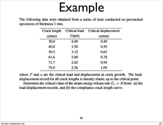
Examples for Fatigue
log
da
dN
= logC + mlogK
K = !p⇡a
5.6 MPapm
17.72 MPapm
da
dN
=
af a0
N
log(xy) = log(x) + log(y)
log(xp) = p log(x)
[Gdoutos]
165

Example
166

Example (Gdoutos p.287)
A large thick plate contains a crack of length 2a₀=10 mm
and is subjected to a constant-amplitude tensile cyclic
stress normal to the crack of which σmin = 100 MPa and
σmax= 200 MPa. The critical SIF is KIc = 60 MPa√m. Fatigue
is governed by the following equation
da
dN
= 0.42 ⇥ 1011(K)3
Plot the crack growth curve--a versus N up to the point
of fracture.
If a lifetime of 106 cycles is required, discuss the option
that the designer has for an improved lifetime.
167
(m/cycle)

200p⇡af = 60 af = 28.65 mm
168
da
dN
= 0.42 ⇥ 1011(!p⇡a)3

Example (Matlab)
A plate of width W=6 in contains a crack of length
2a₀=0.2 in and is subjected to a constant-amplitude tensile
cyclic stress normal to the crack with Δσ=12 ksi. Fatigue
is governed by the following equation
da
dN
= 4⇥ 109(K)3.5
Given
Plot the crack growth curve--a versus N up to the point
of fracture at which the critical crack length 2ac = 5.6 in.
For 2a₀=1 in, do the same and plot the two curves on
the same figure to see the influence of a₀.
169

Summary
!res =
Kc
f(a/W)p⇡a
• What is the residual strength as a function of crack size?
• What is the critical crack size?
• How long does it take for a crack to grow from a certain
initial size to the critical size?
170
f(ac/W)!p⇡ac = Kc
N = N0 +
Z ac
a0
da
C(!p⇡a)m

Mixed-mode crack growth
Combination of mode-I, mode-II and mode-III loadings:
mixed-mode loading.
Cracks will generally propagate along a curved
surface as the crack seeks out its path of least
resistance.
Only a 2D mixed-mode loading (mode-I and mode-II) is
discussed.
171

Maximum circumferential
stress criterion
Erdogan and Sih
(from M. Jirasek) principal stress ⌧r✓ = 0
172

stress criterion
✓c = 2arctan
1
4
⇣
KI/KII ±
⌘
p
(KI/KII)2 + 8
KI
✓
sin
✓
2
+ sin
3✓
2
◆
+ KII
✓
cos
✓
2
+ 3 cos
3✓
2
◆
⌧r✓ = 0 = 0
173

stress criterion Fracture criterion Keq KIc

Experiment
XFEM
✓c = 2arctan
1
4
⇣
KI/KII ±
⌘
p
(KI/KII)2 + 8
175

Ductile to Brittle transition
Fractures occurred in “well-designed”
steel structures in severe
weather.
At low temperatures some metals that would be ductile at room
temperature become brittle. This is known as a ductile to brittle
transition.
As a result, some steel structures are every
likely to fail in winter.
Titanic in the icy water of
Atlantic
176

Stress corrosion cracking
• Metals are subject to corrosion
• Stress corrosion cracking (SCC): interaction of corrosion and
mechanical loadings to produce a cracking failure
• Fracture type: brittle!!!
• Stress corrosion cracking is generally considered to be the most
complex of all corrosion type
corrosive environments
177

Alternatives to LEFM
• Bodies with at least one existing crack
• Nonlinear zone ahead of the crack tip is
negligible
Alternatives:
• Continuum damage mechanics
• Cohesive zone models
• Peridynamics
• Lattice models
crack growth
crack
initiation/
formation
discussed
178

Fracture mechanics for
concrete
179

Introduction
• LEFM theory was developed in 1920, but not until
1961 was the first experimental research in concrete
performed.
• Fracture mechanics was used successfully in
design for metallic and brittle materials early
on; however comparatively few applications
were found for concrete.
• This trend continued up until the middle ‘70s
when finally major advances were made.
• Experimentally observed size-effect can only
be explained using fracture mechanics
180

Tensile response of concrete
• Tensile behavior of concrete is usually ignored: tensile strength is small
• This prevented the efficient use of concrete
• Tensile behavior plays a key role in understanding fracture of concrete
L
! ✏m
quasi-brittle
181
✏m =
L
L
= ✏0 +
w
L
L

Fictitious crack model
Fracture Process Zone (FPZ)
concrete=quasi-brittle material
182

Hilleborg’s fictitious
1976 crack model
Cohesive crack/zone model
Similar to the strip yield model of Dugdale-Barenblatt
183

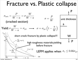
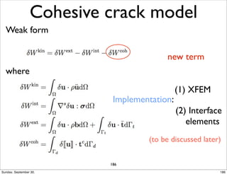
Cohesive crack model
G =
Z
([[u]])d[[u]]
Fracture criterion
1
2
when
max ft
where (direction)
Rankine criterion

Governing equations
(strong form)
Constitutive equations
deformation
separation
185

Weak form
where
186

Weak form
new term
where
186

Weak form
new term
Implementation:
(1) XFEM
(2) Interface
elements
(to be discussed later)
where
186

Size effect
• Experiment tests: scaled versions of real structures
• The result, however, depends on the size of the
specimen that was tested
• From experiment result to engineering design:
knowledge of size effect required
• The size effect is defined by comparing the nominal
strength (nominal stress at failure) N
of geometrically
similar structures of different sizes.
• Classical theories (elastic analysis with allowable
stress): cannot take size effect into account
187pa

• Size effect is crucial in concrete structures (dam,
bridges), geomechanics (tunnels): laboratory tests
are small
• Size effect is less pronounced in mechanical and
aerospace engineering the structures or structural
components can usually be tested at full size.
geometrically similar structures
of different sizes
N =
cNP
bD b is thickness
188

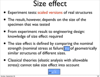
Structures and tests
[Dufour]
189

Size effect (cont.)
1. Large structures are softer than small structures.
2. A large structure is more brittle and has a lower
strength than a small structure.
190

Bazant’s size effect law
N = ft = ft(D)0
!N =
KIc p⇡a
=
KIc p⇡cND
For very small structures the curve approaches the horizontal line and, therefore, the
failure of these structures can be predicted by a strength theory. On the other hand,
for large structures the curve approaches the inclined line and, therefore, the failure
of these structures can be predicted by LEFM.
191

Bazant’s size effect law
192

Continuum damage mechanics
nominal stress
effective stress
Equilibrium: A = ¯A¯
damage variable
Hook’s law:
Milan Jirasek
! =
A¯
A
¯! = (1 !)¯!, ! = 1
A¯
A
¯! = E
= (1 !)E
¯
A
A¯

193

Four point bending test
194

Numerical solution with
CDM
Experiment
Single Edged Notch Beam
(SEN beam)
195

Computational
fracture mechanics
196

Numerical methods to
solve PDEs
• FEM (Finite Element Method)
• BEM (Boundary Element Method)
• MMs (Meshless/Meshfree methods)
FEM
BEM
MMs
197

Fracture models
• Discrete crack models (discontinuous
models)
- LEFM (FEM,BEM,MMs)
- EPFM (FEM,MMs)
- Cohesive zone models (FEM,XFEM,MMs)
• Continuous models
- Continuum damage models (FEM,XFEM)
- Phase field models (FEM)
• Lattice models (FEM)
• Peridynamic models (FEM,MMs)
198

FEM for elastic cracks
(1) double nodes
(2) singular
• Developed in 1976 (Barsoum)
• double nodes: crack edge
• singular elements: crack tip
• remeshing as crack grows
(3) remeshing elements
1
pr behavior
199

What’s wrong with FEM for
crack problems
• Element edges must conform to the crack geometry:
make such a mesh is time-consuming, especially for 3D
problems.
• Remeshing as crack advances: difficult
200

However ...
Bouchard et al. CMAME 2003
Show crack growth movies
201

202

Extended Finite Element
Method (XFEM)
Belytschko et al 1999 Sc set of enriched nodes
uh(x) =
X
I2S
NI (x)uI +
X
J2Sc
NJ (x)(x)aJ
standard part enrichment part
Partition of Unity (PUM) enrichment function
X
J
NJ (x) = 1
X
J
NJ (x)(x) = (x)
(x)
known characteristics of the problem (crack tip singularity,
displacement jump etc.) into the approximate space.
203

XFEM: enriched nodes
nodal support
I
enriched nodes = nodes whose support is cut by the item
to be enriched
enriched node I: standard degrees of uI
freedoms
(dofs) and additional aI
dofs
NI (x)6= 0
X
J
NJ (x)(x) = (x)
204

XFEM for LEFM
u =
KI
2μ
r
r
2⇡
cos
✓
2
✓
 1 + 2 sin2 ✓
2
◆
v =
KI
2μ
r
r
2⇡
sin
✓
2
✓
 + 1 2 cos2 ✓
2
◆
crack tip with known
displacement
crack edge displacement: discontinuous across
crack edge
x+
x
1 = f(pr, ✓)
2 : 2(x+)6= 2(x)
205

H(x) =
⇢
+1 if (x − x⇤) · n 0
−1 otherwise
u =
KI
2μ
r
r
2⇡
cos
✓
2
✓
 1 + 2 sin2 ✓
2
◆
v =
KI
2μ
r
r
2⇡
sin
✓
2
✓
 + 1 2 cos2 ✓
2
◆
XFEM for LEFM (cont.)
Sc
St
blue nodes
red nodes
Crack tip enrichment functions:
[B↵] =

pr sin
✓
2
,pr cos
✓
2
,pr sin
✓
2
sin ✓,pr cos
✓
2
sin ✓

Crack edge enrichment functions:
+
X
K2St
NK(x)
X4
↵=1
B↵b↵
K
!
uh(x) =
X
I2S
NI (x)uI
+
X
J2Sc
NJ (x)H(x)aJ
206

Domain form of J-integral
J-integral is a contour integral that is not well suitable
to FE computations.
FE mesh
J =
Z
A⇤

!ij
@uj
@x1 W#1i
#
@q
@xi
dA
207

XFEM for cohesive cracks
Sc
Wells, Sluys, 2001
H(x) =
⇢
+1 if (x − x⇤) · n 0
−1 otherwise
uh(x) =
X
I2S
NI (x)uI +
X
J2Sc
NJ (x)H(x)aJ
No crack tip solution is known, no tip
enrichment!!!
not enriched to ensure zero
crack tip opening!!!
208

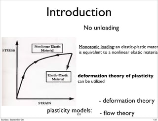
XFEM: SIFs computation
Mesh
Results
One single mesh for all angles!!!
[VP Nguyen Msc. thesis]
Matlab code: free
209

XFEM: examples
CENAERO, M. Duflot
Northwestern Univ.
210

XFEM-Crack propagation
Samtech, Belgium
fracture of underwater
211 gas-filled pipeline

Meshfree methods
Bordas et al.
Elastic-plastic fracture Shaofan Li 2012
212

Interface elements and
cohesive crack model
fracture of polycrystalline material
delamination of composites
213

Dynamic fracture
• Dynamics is much more difficult than static
• Dynamic fracture mechanics
- inertia forces (kinetic energy)
- rate-dependent material behavior
- reflected stress waves
• Classification
- LEFM - Elastodynamic fracture mechanics
214

Crack speed of
215

Interfacial fracture mechanics
• Thin films
•
216

Fracture of composite
materials
217

Fiber reinforced
composites
218

Fracture mechanics

More Related Content

What's hot

Similar to Fracture mechanics

More from Nguyen Vinh Phu

Recently uploaded

Fracture mechanics