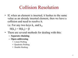
Downloaded 43 times
![4
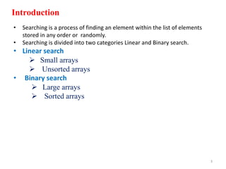
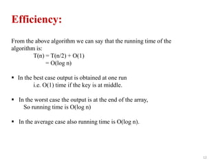
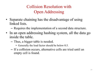
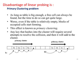
• In linear search, access each element of an array one by one
sequentially and see whether it is desired element or not. A search will
be unsuccessful if all the elements are accessed and the desired element
is not found.
• In brief, Simply search for the given element left to right and return the
index of the element, if found. Otherwise return “Not Found”.
Algorithm:
LinearSearch(A, n,key)
{
for(i=0;i<n;i++)
{
if(A[i] == key)
return i;
}
return -1; //-1 indicates unsuccessful search
}
Analysis: Time complexity = O(n)
Linear Search](https://image.slidesharecdn.com/unit-viiisearchingandhashing-150912062511-lva1-app6892/85/Unit-viii-searching-and-hashing-4-320.jpg)
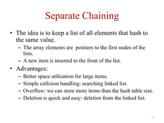
![6
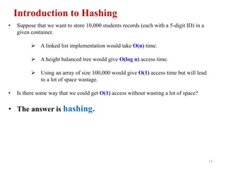
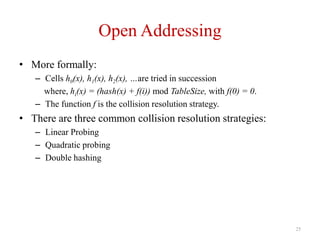
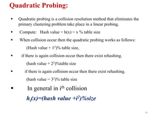
Iterative Algorithm
BinarySearch(A, l, r, key)
{
while(l<=r)
{
m = (l + r) /2 ; //integer division
if(key = = A[m]
print " Search successful"
else if (key < A[m])
r = m - 1
else
l = m+1
}
If(l>r)
print "unsuccessful search"
}](https://image.slidesharecdn.com/unit-viiisearchingandhashing-150912062511-lva1-app6892/85/Unit-viii-searching-and-hashing-6-320.jpg)
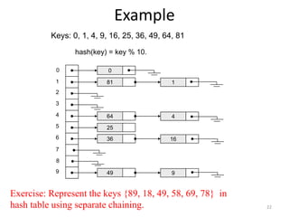
![7
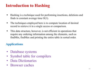
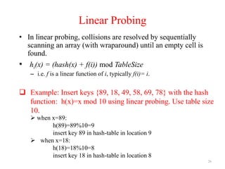
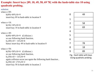
Algorithm: Recursive
BinarySearch(A, l, r, key)
{
if(l= = r) //only one element
{
if(key = = A[l])
print " successful Search"
else
print "unsuccessful Search"
}
else
{
m = (l + r) /2 ; //integer division
if(key = = A[m]
print "successful search"
else if (key < A[m])
return BinarySearch(l, m-1, key) ;
else
return BinarySearch(m+1, r, key) ;
}
}](https://image.slidesharecdn.com/unit-viiisearchingandhashing-150912062511-lva1-app6892/85/Unit-viii-searching-and-hashing-7-320.jpg)
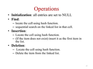
![9
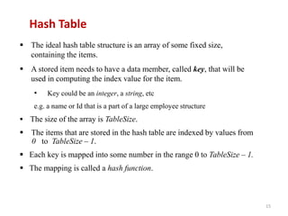
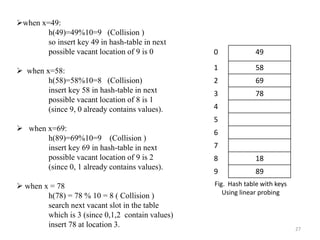
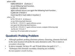
Running example:
Take input array a[]
For Search key = 2
l r mid remarks
0 13 6 Key < a[6] i.e. 2 < 53
0 5 2 Key < a[2] i.e. 2 < 7
0 1 0 Key == a[0] i.e. 2 ==a[0]
Therefore, key found at index 0.
Search Successful !!
2 5 7 9 18 45 53 59 67 72 88 95 101 104
0 1 2 3 4 5 6 7 8 9 10 11 12 13
Exercise : Trace binary search algorithm for keys:
i. 67
ii. 50
iii. 250](https://image.slidesharecdn.com/unit-viiisearchingandhashing-150912062511-lva1-app6892/85/Unit-viii-searching-and-hashing-9-320.jpg)
![10
Search for key = 67
l r mid Remarks
0 13 6 Key < a[6] i.e. 67 > 53
7 13 10 Key < a[10] i.e. 67 < 88
7 9 8 Key == a[8] i.e. 67 ==a[8]
Therefore, key found at index 8.
Search Successful !!
2 5 7 9 18 45 53 59 67 72 88 95 101 104
0 1 2 3 4 5 6 7 8 9 10 11 12 13
Input Array : a[ ]](https://image.slidesharecdn.com/unit-viiisearchingandhashing-150912062511-lva1-app6892/85/Unit-viii-searching-and-hashing-10-320.jpg)
![11
Search for key = 50
l r mid Remarks
0 13 6 Key < a[6] i.e. 50 < 53
0 5 2 Key < a[2] i.e. 50 > 7
3 5 4 Key > a[4] i.e. 50 >18
5 5 5 Key > a[5] i.e. 50 > 45
6 5 l > r, terminate
Therefore, key not found in the array.
Search Unsuccessful !!
2 5 7 9 18 45 53 59 67 72 88 95 101 104
0 1 2 3 4 5 6 7 8 9 10 11 12 13
Given Input Array a[]](https://image.slidesharecdn.com/unit-viiisearchingandhashing-150912062511-lva1-app6892/85/Unit-viii-searching-and-hashing-11-320.jpg)
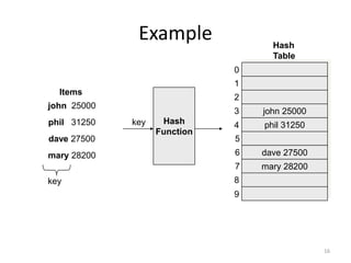
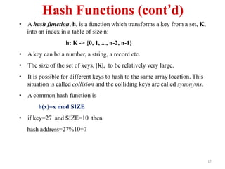
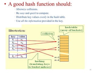
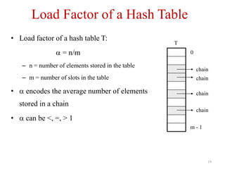
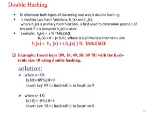
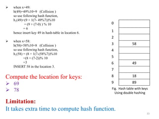


Unit – VIII discusses searching and hashing techniques. It describes linear and binary searching algorithms. Linear search has O(n) time complexity while binary search has O(log n) time complexity for sorted arrays. Hashing is also introduced as a technique to allow O(1) access time by mapping keys to array indices via a hash function. Separate chaining and open addressing like linear probing and quadratic probing are described as methods to handle collisions during hashing.