The document discusses searching techniques in data structures, distinguishing between linear (sequential) and binary search methods. It describes key search terminologies and algorithms, emphasizing the efficiency of binary search in sorted lists compared to linear search in unsorted lists. Additionally, it introduces hashing as a method to optimize search processes, explaining hash functions, hash tables, and collision resolution techniques.

1. 10/8/2023
Data Structure & Algorithm
Unit-III Searching
by:
Dr. Shweta Saraswat

2. 10/8/2023
Contents
Searching Techniques:

3. SEARCHING

4. Introduction
4
• Search can be viewed abstractly as a process
to determine if an element with a particular
value is a member of a particular set.
• Searching refers to finding out whether a particular
element is present in the list or not.
• Search algorithms are algorithms that find one
element of a set by some key containing other
information related to the key.
• If the list is an unordered list, then we use linear or
sequential search, whereas if the list is an ordered
list, then we use binary search.

5. 5
Searching Terminologies
• Internal key
• Key is contained within the record at a specific offset
from the start of the
record
• External Key
• There is a separate table of keys that includes pointers
to the records
• Primary Key
• The key used to search is unique for every record in
the table
• Secondary Key
• Same key may be associated with more than one
record in the table

6. 6
Searching Terminologies
• Search algorithm
• Accepts an argument and tries to find a record in a given
table whose key it matches
• Successful search
• Algorithm finds at least one record
• Unsuccessful search
• Algorithm doesn’t find any records
• Retrieval
• A successful search is often called retrieval
• Internal Searching
• Records to be searched are sorted entirely within computer
main memory
• External Searching
• For large records we need external storage devices and we
search on such devices.

7. 7
Searching Algorithms
• Basically there are two categories of
searching algorithms
Sequential Search or Linear Search
Binary Search

8. 8
Linear or Sequential Search
• This the simplest method for searching, in this method the
element to be found is searched sequentially in the list.
• This method can be used on a sorted or an unsorted list.
• In case of a sorted list searching starts from 0th element
and continues until the element is found or the element
whose value is greater than the value being searched is
reached
• Searching in case of unsorted list starts from the 0th
element and continues until the element is found or the
end of the list is reached.

9. Linear or Sequential Search
• The list given above is the list of elements in an
unsorted array.
• The array contains 10 elements, suppose the
element to be searched is 46 then 46 is compared
with all the elements starting from the 0th element
and searching process ends where 46 is found or
the list ends.
• The performance of the linear search can be
measured by counting the comparison done to
find out an element.
• The number of comparisons is 0(n) 9

10. 1
0
Binary Search
• Binary search technique is very fast and efficient. It requires the list of the
elements to be in sorted order.
• The logic behind this technique is given below:
• First find the middle element of the array
• compare the middle element with an item.
• There are three cases:
• If it is a desired element then search is successful
• If it is less than desired item then search only the first half of
the array.
• If it is greater than the desired element, search in the second
half of the array.
• Repeat the same process until element is found or exhausts in the search
area.
• In this algorithm every time we are reducing the search area.
• We can apply binary search technique recursively or iteratively

11. Recursive Binary Search
• As the list is divided into two halves, searching begins
• Now we check if the searched item is greater or less
than the center element.
• If the element is smaller than the center element then the
searching is done in the first half, otherwise it is done in
the second half
• The process is repeated till the element is found or the
division of half parts gives one element.

12. 1
2
Recursive Binary Search
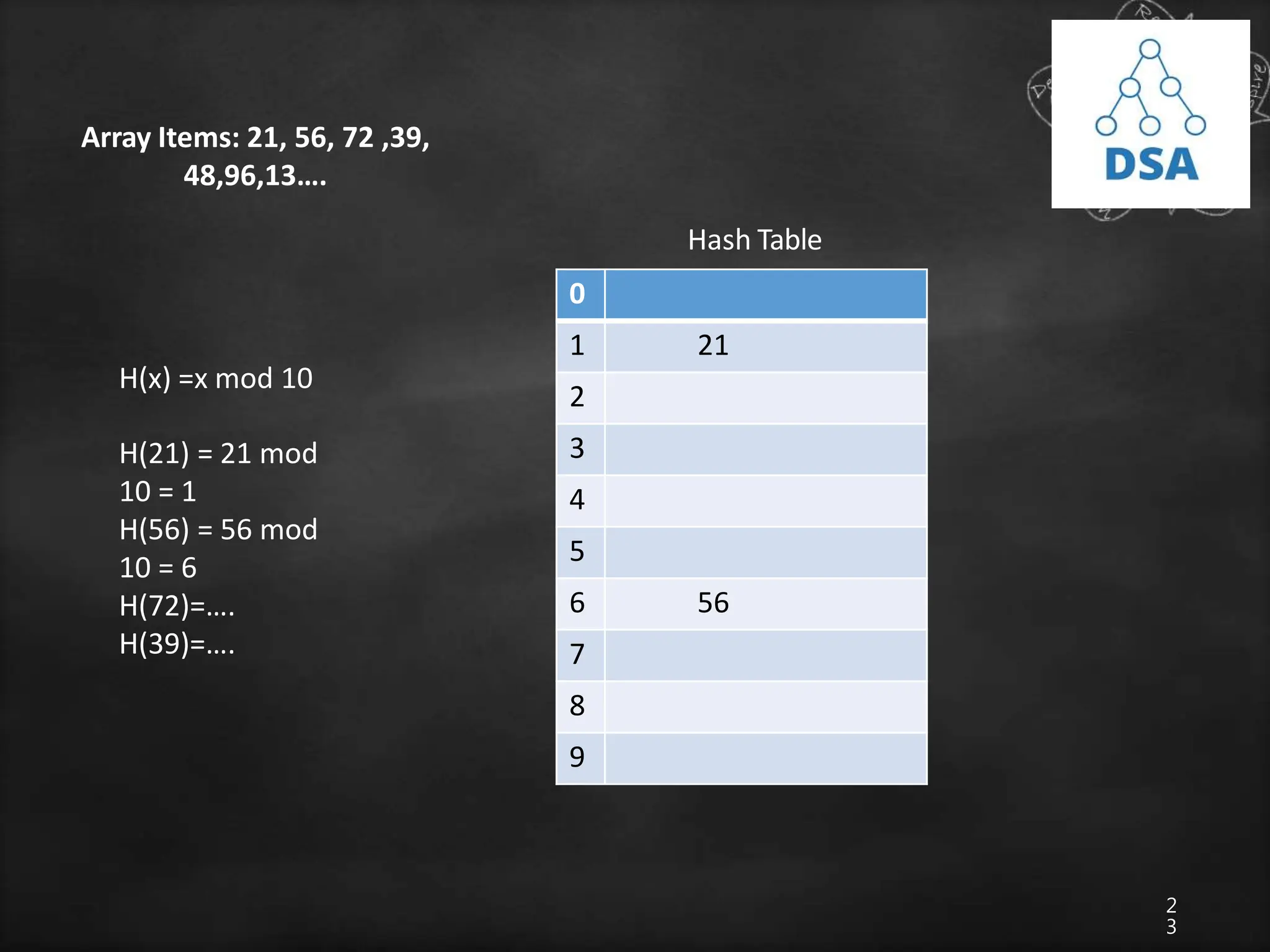
• Let a[n] be a sorted array of size n and x be an item
to be searched. Let low=0 and high=n-1 be lower
and upper bound of an array
1. If (low>high)
return 0;
2. mid=(low+high)/2;
3. if (x==a[mid])
4. Return mid;
5. If (x<a[mid])
Search for x in a[low] to a[mid-1];
5. else
Search for x in a[mid+1] to a[high];

13. 1
3
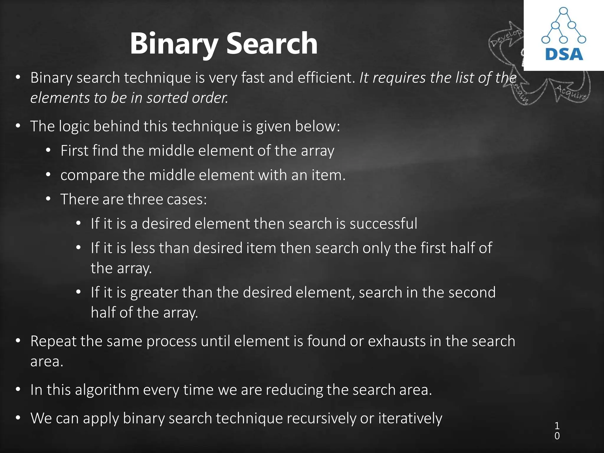
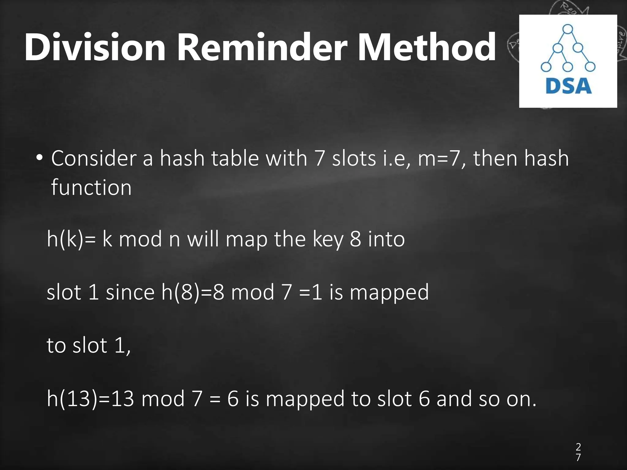
• We need to search 46, we can assign first=0 and last= 9 since
first and last are the initial and final position/index of an array
• The binary search when applied to this array works as
follows:
1. Find center of the list i.e. (first+last)/2 =4 i.e. mid=array[4]=10
2. If higher than the mid element we search only on the upper half
of an array
else search lower half. In this case since 46>10, we search the
upper half
i.e. array[mid+1] to array [n-1]
3. The process is repeated till 46 is found or no further subdivision
of array is possible
0 1 2 9 10 11 15 20 46 72

14. Ashim
Lamichhane
1
4

15. 1
5
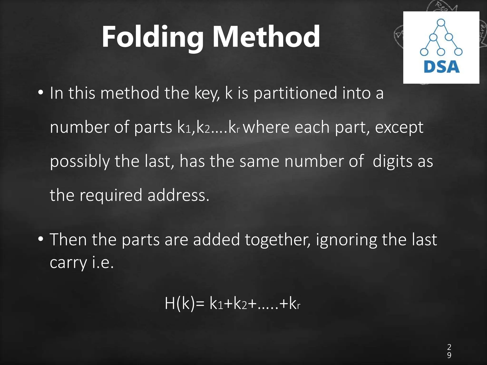
Iterative Binary Search Algorithm
• The recursive algorithm is inappropriate in practical
situations in which efficiency is a prime
consideration.
• The non-recursive version of binary search algorithm
is given below.
• Let a[n] be a sorted array with size n and key is an
item being searched for.

16. 1
6
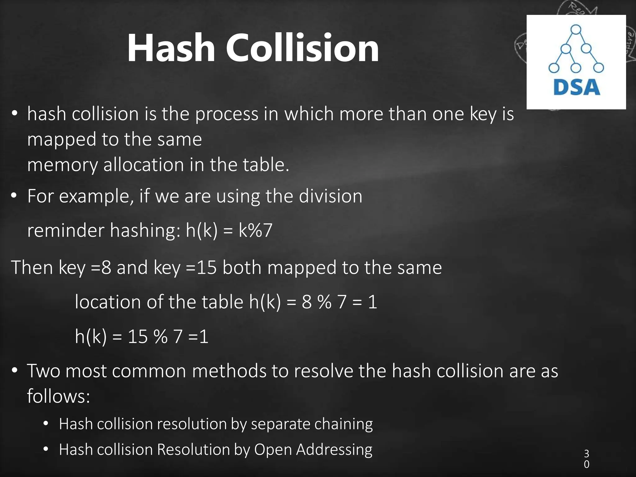
Algorithm
low=0; hi=n-1; while(low<=hi){
mid=(low+hi)/2; if(key==a[mid])
return mid; if (key<a[mid])
hi=mid-1;
else
low=mid+1;
}
return 0;

17. 1
7

18. 1
8
Comparison of sequential and
binary search algorithm
Sequential Search Binary Search
Time complexity: 0(n) Time complexity: 0(logn)
Only eliminates one element from
the search per comparison
Eliminates half of the array
elements for each comparison
As n number of elements gets very large,
sequential
search has to do lot more work
As n number or elements gets very large,
binary
search has to do little work than
sequential search
Has to search each element
i,i+1,i+2,i+3…….n
Has to search n/2,n/4,n/8….1 elements
Doesn’t require element to be in sorted
order
Requires elements to be in sorted order
Easy to program but takes too much time Easy to program and execution time
faster

19. 1
9
Application of Search
Algorithms
• Search Engines
• Online enquiry
• Text Pattern
matching
• Spell Checker
• Ant algorithm

20. 2
0
Hashing Intro
• Now the only problem at hands is to speed up searching.
• Consider a problem of searching an array for a given value.
• If array is not sorted, need to search each and every elements
• If array is sorted, binary search whose worse-case runtime
complexity 0(logn)
• We could search even faster if we know in advance the index
at which that value is located in the array.
• We could use some magic function where our search
would be reduced to a constant runtime 0(1). Such
magic function is called hash function.
• A hash function is a function which when given a key,
generates an address in the table

21. 2
1
Hashing
• The process of mapping large amounts of data
into a smaller table is called hashing.
• Hashing is relatively easy to program as compared to
tree however it is based on arrays, hence difficult to
expand
• It performs insertions, deletions and finds in
constant average time.

22. 2
2
Hash Table
• A hash table is a data structure where we store a key value after
applying the hash
function, it is arranged in the form of an array that is
addressed via a hash function.
• The hash table is divided into number of buckets and each
bucket is in turn capable of storing a number of record.
• Thus we can say that a bucket has a number of slots and each
slot is capable of holding one record
• The time required to locate any element in the hash table is 0(1).
• Now the question may arise how do we map number of keys
to a particular location in the hash table. i.e. h(k). It is
computed using hash function

23. 2
3
0
1 21
2
3
4
5
6 56
7
8
9
Hash Table
Array Items: 21, 56, 72 ,39,
48,96,13….
H(x) =x mod 10
H(21) = 21 mod
10 = 1
H(56) = 56 mod
10 = 6
H(72)=….
H(39)=….

24. 2
4
Hash Function
• A function that transforms a key into a table index is called a hash
function
• If h is a hash function and k is a key) is called the hash of key and
is the index in which a record with the key k should be placed.
• The basic idea in hashing is the transformation of a key into the
corresponding location in
the hash table. This is done by hash function.
• It is usually denoted by H
H: K -> M
where, H=hash function
K= set of keys
M=set of memory
address

25. 2
5
Hash Functions
• Sometimes, such function H may not yield distinct values, It
is possible that two
different keys K1 and K2 will yield the same hash address.
• This situation is called Hash Collision
• To choose the hash function H:K->M there are two things to
consider.
• First the function H should be very easy and quick to compute.
• Second, H should distribute the keys to the number of location of
hash table with less no of collisions
• Some hash functions:
• Division reminder method
• Mid square method
• Folding method

26. 2
6
Division Reminder Method
• In this method, key k is divided by a number m larger
than the number n or keys in k and the reminder of this
division is taken as index into the hash table i.e.
h(k)=k mod m
• The number m is usually chosen to be a prime number
or a number without small divisors, since this
frequently minimizes the number of collisions

27. 2
7
Division Reminder Method
• Consider a hash table with 7 slots i.e, m=7, then hash
function
h(k)= k mod n will map the key 8 into
slot 1 since h(8)=8 mod 7 =1 is mapped
to slot 1,
h(13)=13 mod 7 = 6 is mapped to slot 6 and so on.

28. 2
8
Mid Square Method
• In this method the key is first squared. Therefore the hash
function is defined by h(k) =p,
where p is obtained by deleting digits from both sides of k2.
• To implement this the same position of k2 must be used for all the
keys.
• Ex: consider a hash table with 50 slots i.e m=50 and key values k
=1632,1739,3123.
• Solution:
k = 1632
k2 = 2663424
h(k) = 34

29. 2
9
Folding Method
• In this method the key, k is partitioned into a
number of parts k1,k2….kr where each part, except
possibly the last, has the same number of digits as
the required address.
• Then the parts are added together, ignoring the last
carry i.e.
H(k)= k1+k2+…..+kr

30. 3
0
Hash Collision
• hash collision is the process in which more than one key is
mapped to the same
memory allocation in the table.
• For example, if we are using the division
reminder hashing: h(k) = k%7
Then key =8 and key =15 both mapped to the same
location of the table h(k) = 8 % 7 = 1
h(k) = 15 % 7 =1
• Two most common methods to resolve the hash collision are as
follows:
• Hash collision resolution by separate chaining
• Hash collision Resolution by Open Addressing

31. 3
1
Hash collision resolution by
separate chaining
• In this method all the elements where keys hash
to the same hash- table slot are put in one linked
list
• Therefore the slot in the hash table contains a
pointer to the head of the linked list

32. 3
2
Hash collision Resolution by
Open Addressing
• In open addressing the keys to be hashed is to put in the separate
location of the
hash table.
• Each location contains some key or the some other character to
indicate that the
particular location is free
• Some popular methods
• Linear probing
• Quadratic probing
• Double Hashing
• Rehashing

33. Ashim
Lamichhane
3
3
Linear probing
• A hash-table in which a collision is resolved by
putting the item in the next empty place within the
occupied array space
• It starts with a location where the collision occurred
and does a sequential search through a hash table
for the desired empty location
• Hence the method searches in straight line, and it
is therefore called linear probing.

34. • Example: insert keys {89,18,49,58,69} with the
hash function h(x) = x mod 10 using linear probing
3
4

35. 3
5
Quadratic probing
• Quadratic probing is a collision resolution method that
eliminates the primary collision
problem.
• When collision occur then the quadratic
probing works as follows: (Hash value +12)
% tablesize
• If there is again collision
then there exist rehashing
(Hash value +22) % tablesize
• If there is again collision then there exist rehashing
(Hash value +32) % tablesize
• Same goes again, in ith collision
h(x) =(hash value + i2) % tablesize

36. 3
6