Quicksort has average time complexity of O(n log n), but worst case of O(n^2). It has O(log n) space complexity for the recursion stack. It works by picking a pivot element, partitioning the array into sub-arrays of smaller size based on element values relative to the pivot, and recursively
Unit 5
Internal Sorting& Files
Dr. R. Khanchana
Assistant Professor
Department of Computer Science
Sri Ramakrishna College of Arts and Science for
Women
http://icodeguru.com/vc/10book/books/book1/chap07.htm
http://icodeguru.com/vc/10book/books/book1/chap10.htm
Tutorials :
https://www.tutorialspoint.com/data_structures_algorithms/insertion_sort_algorithm.htm
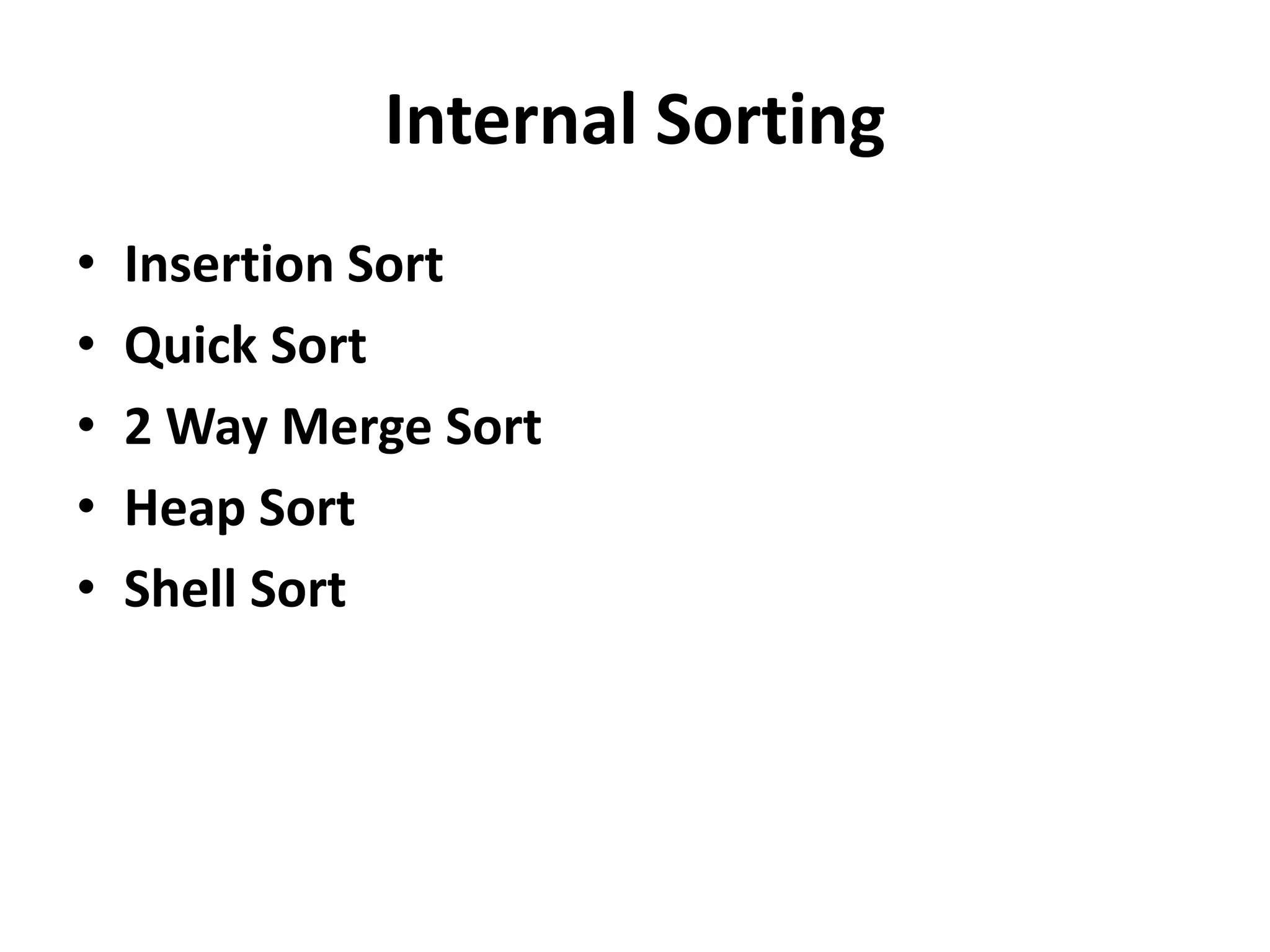
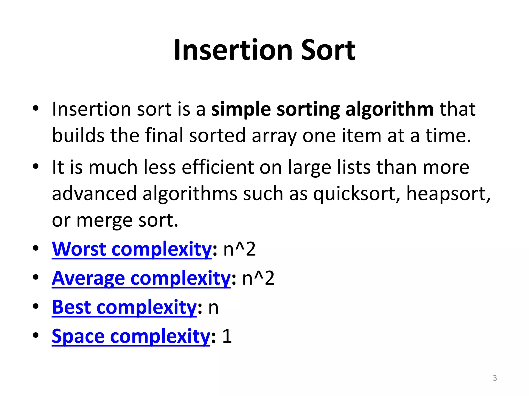
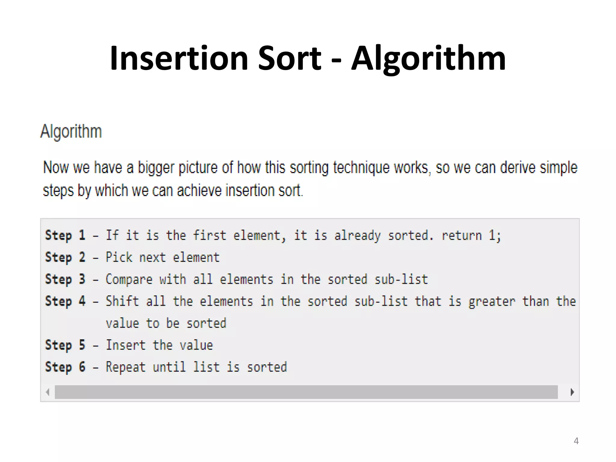
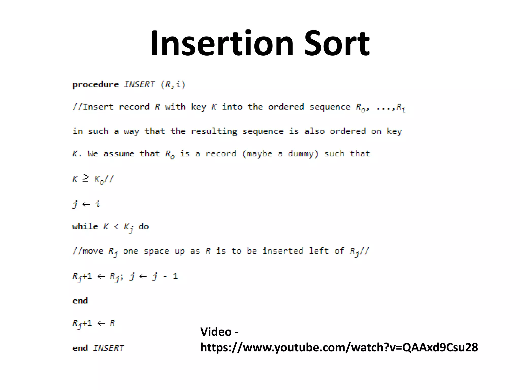
Insertion Sort
• Insertionsort is a simple sorting algorithm that
builds the final sorted array one item at a time.
• It is much less efficient on large lists than more
advanced algorithms such as quicksort, heapsort,
or merge sort.
• Worst complexity: n^2
• Average complexity: n^2
• Best complexity: n
• Space complexity: 1
3
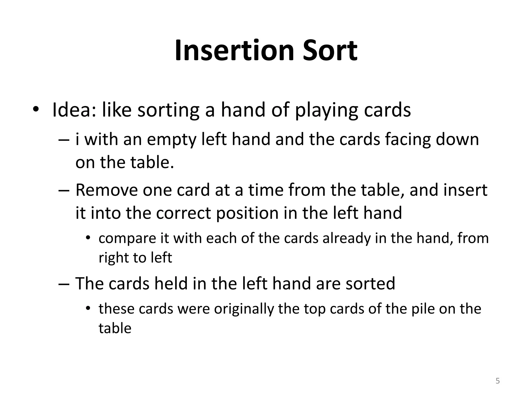
Insertion Sort
• Idea:like sorting a hand of playing cards
– i with an empty left hand and the cards facing down
on the table.
– Remove one card at a time from the table, and insert
it into the correct position in the left hand
• compare it with each of the cards already in the hand, from
right to left
– The cards held in the left hand are sorted
• these cards were originally the top cards of the pile on the
table
5
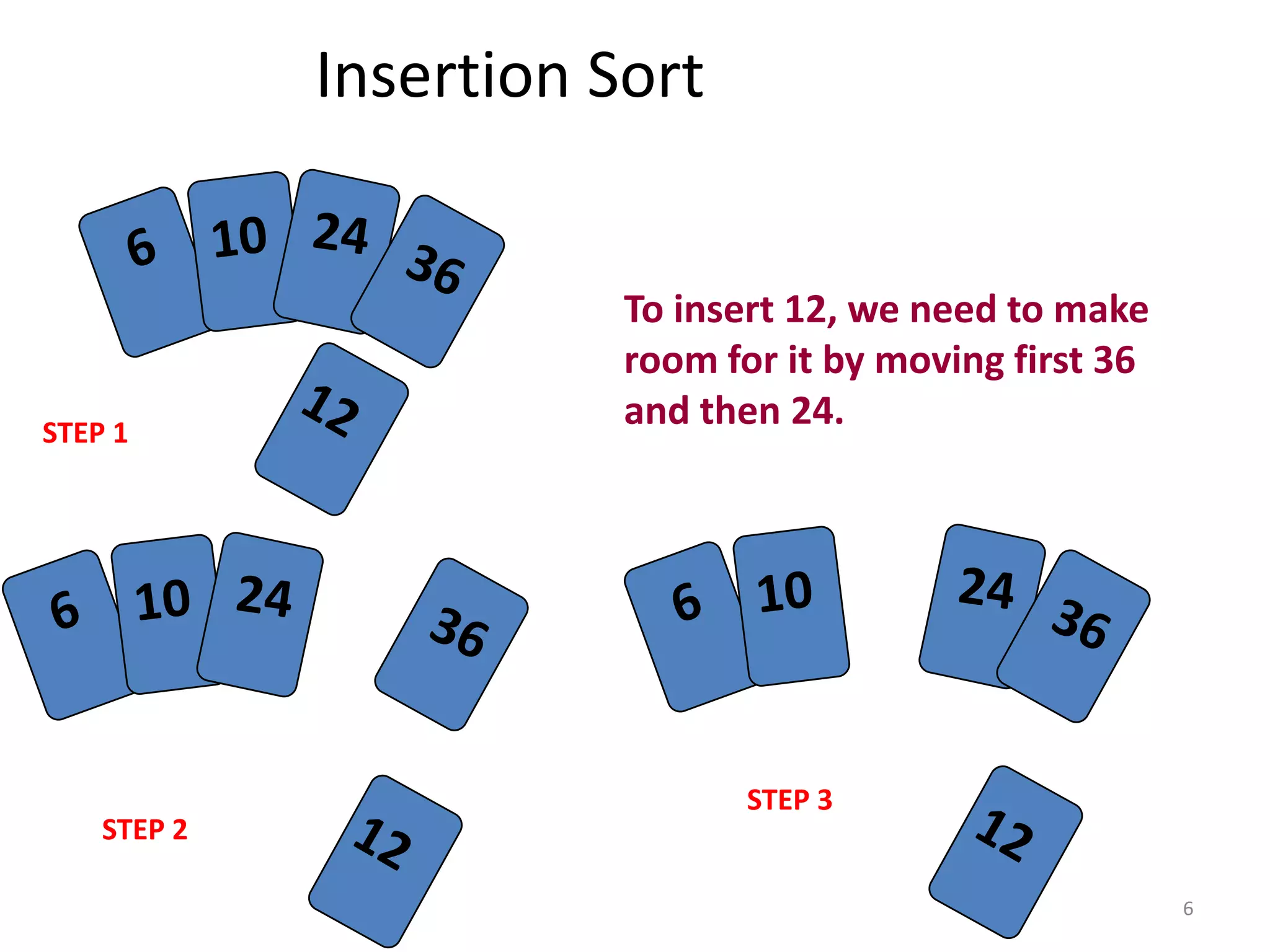
6.
Insertion Sort
6
To insert12, we need to make
room for it by moving first 36
and then 24.STEP 1
STEP 2
STEP 3
7.
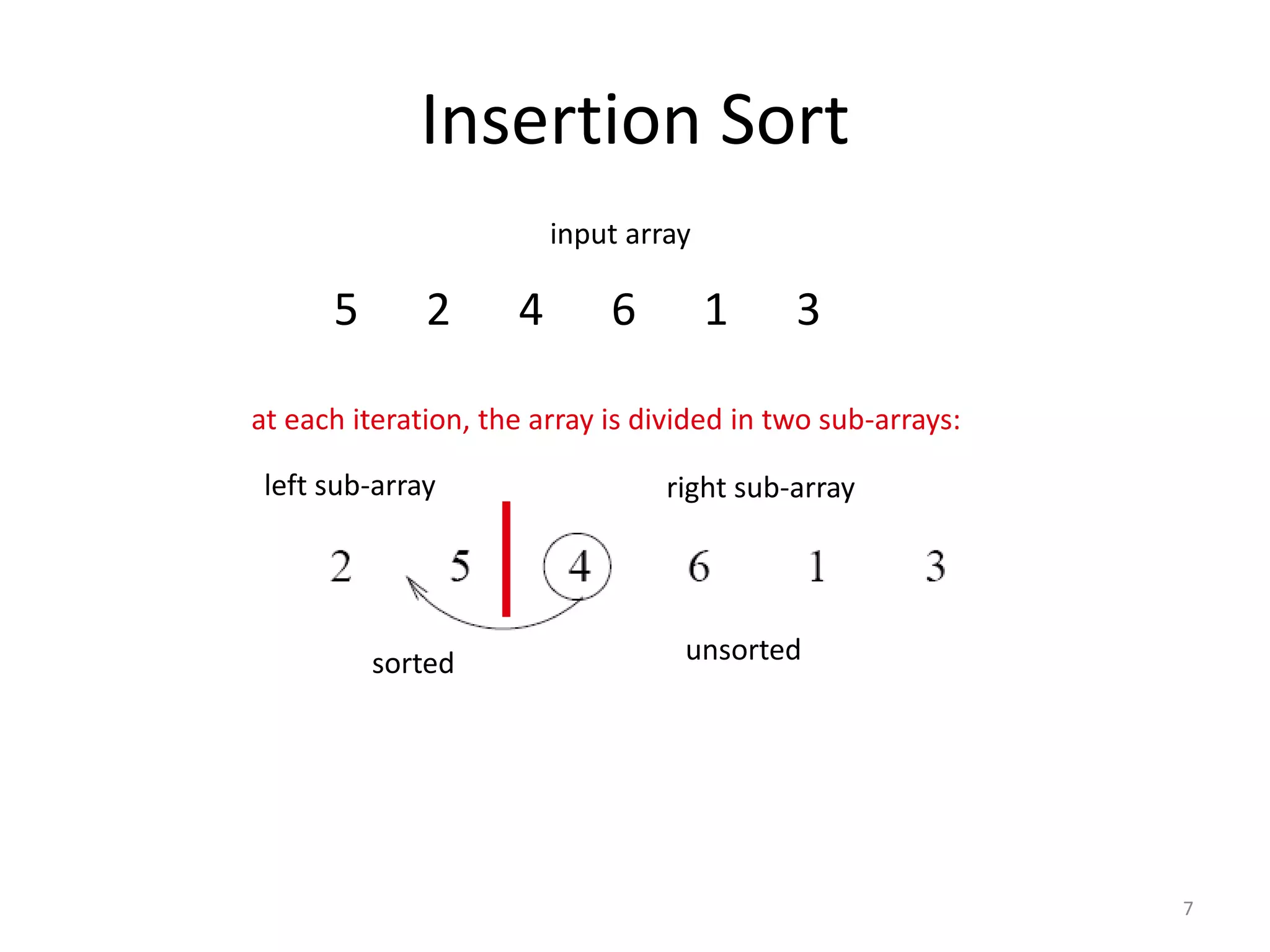
Insertion Sort
7
5 24 6 1 3
input array
left sub-array right sub-array
at each iteration, the array is divided in two sub-arrays:
sorted unsorted
Insertion Sort
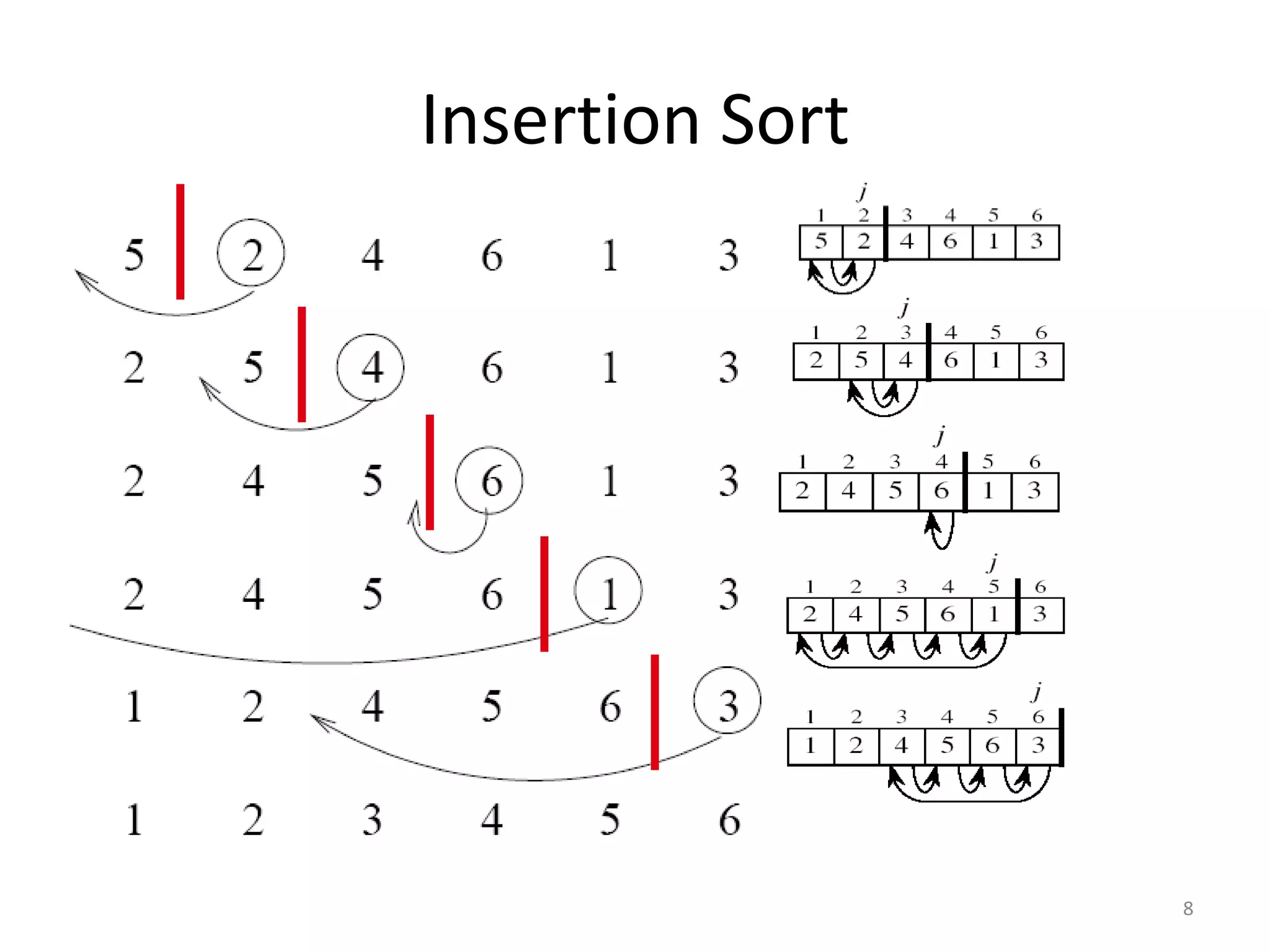
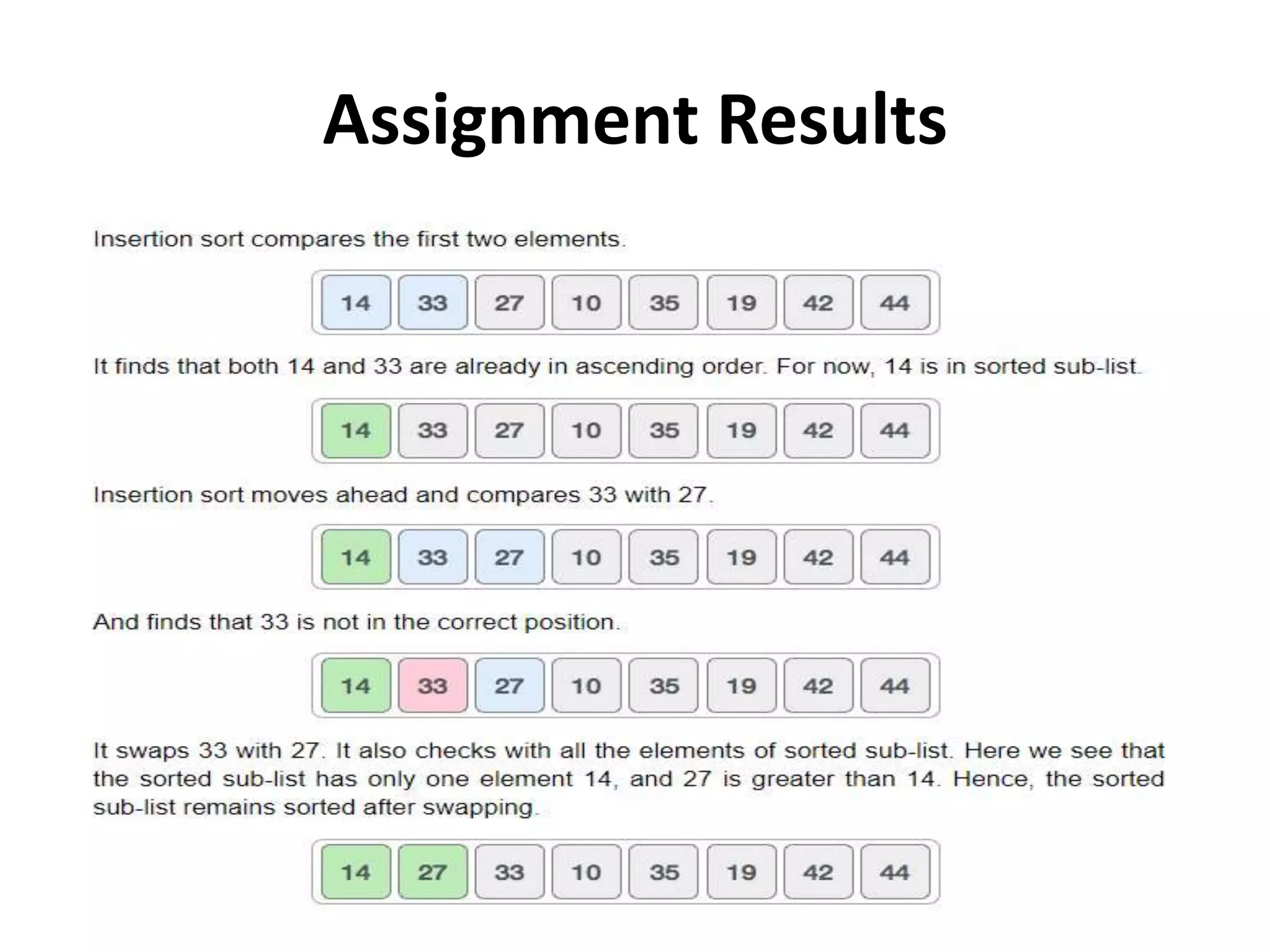
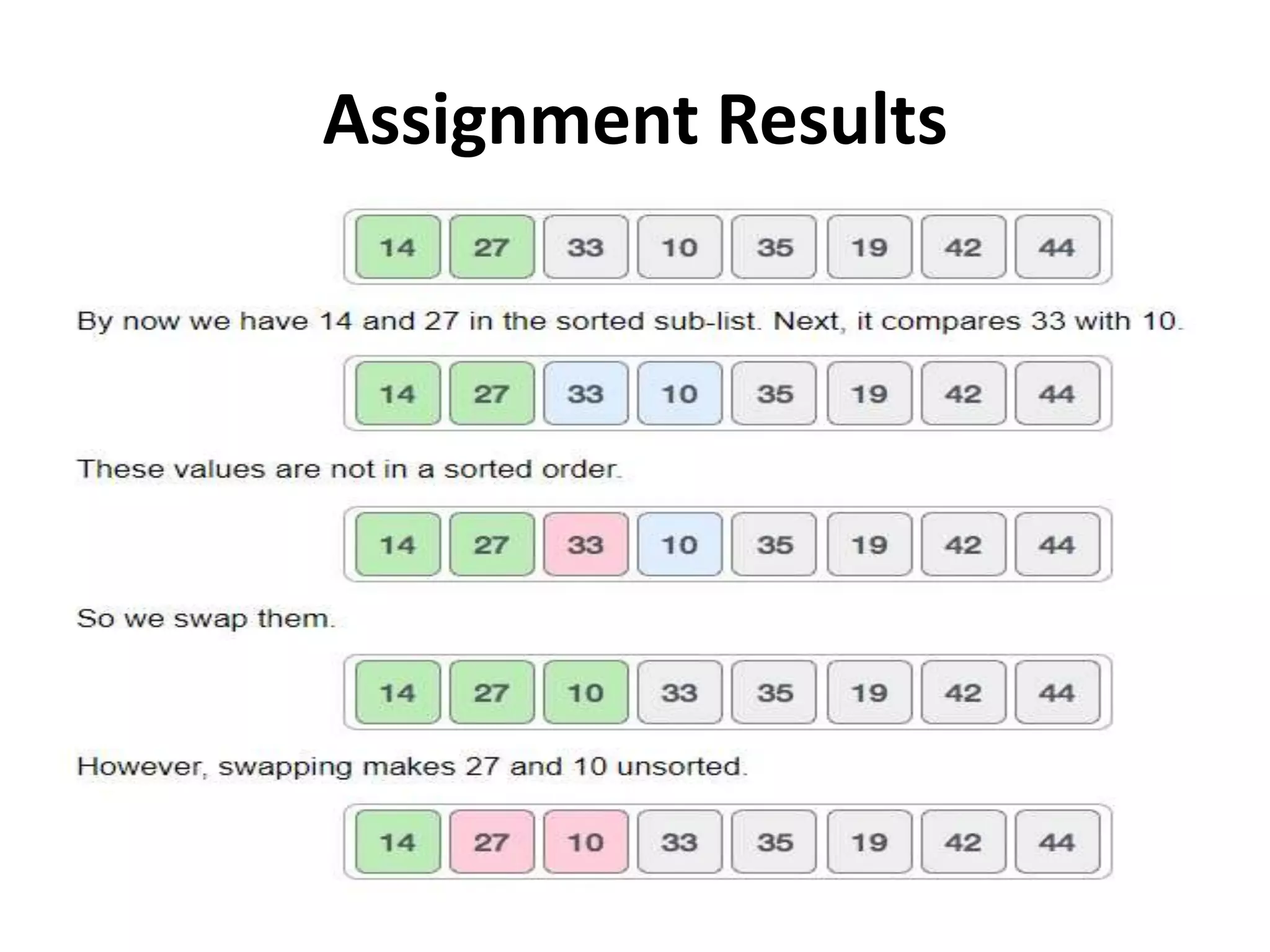
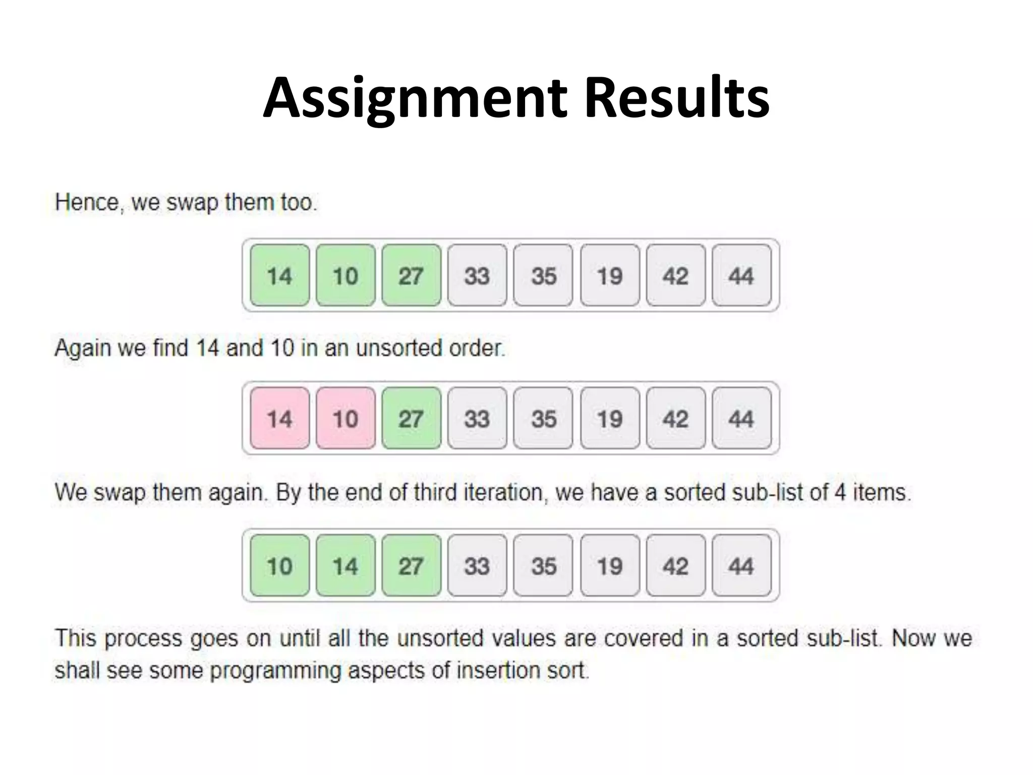
• Example7.1: Assume n = 5 and the input sequence is (5,4,3,2,1) [note the
records have only one field which also happens to be the key]. Then, after
each insertion we have the following:
Note that this is an example of the worst case behavior.
• Example 7.2: n = 5 and the input sequence is (2, 3, 4, 5, 1). After each
execution of INSERT we have:
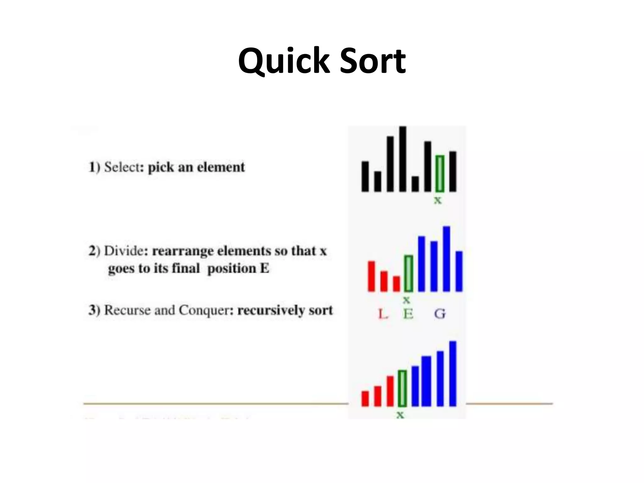
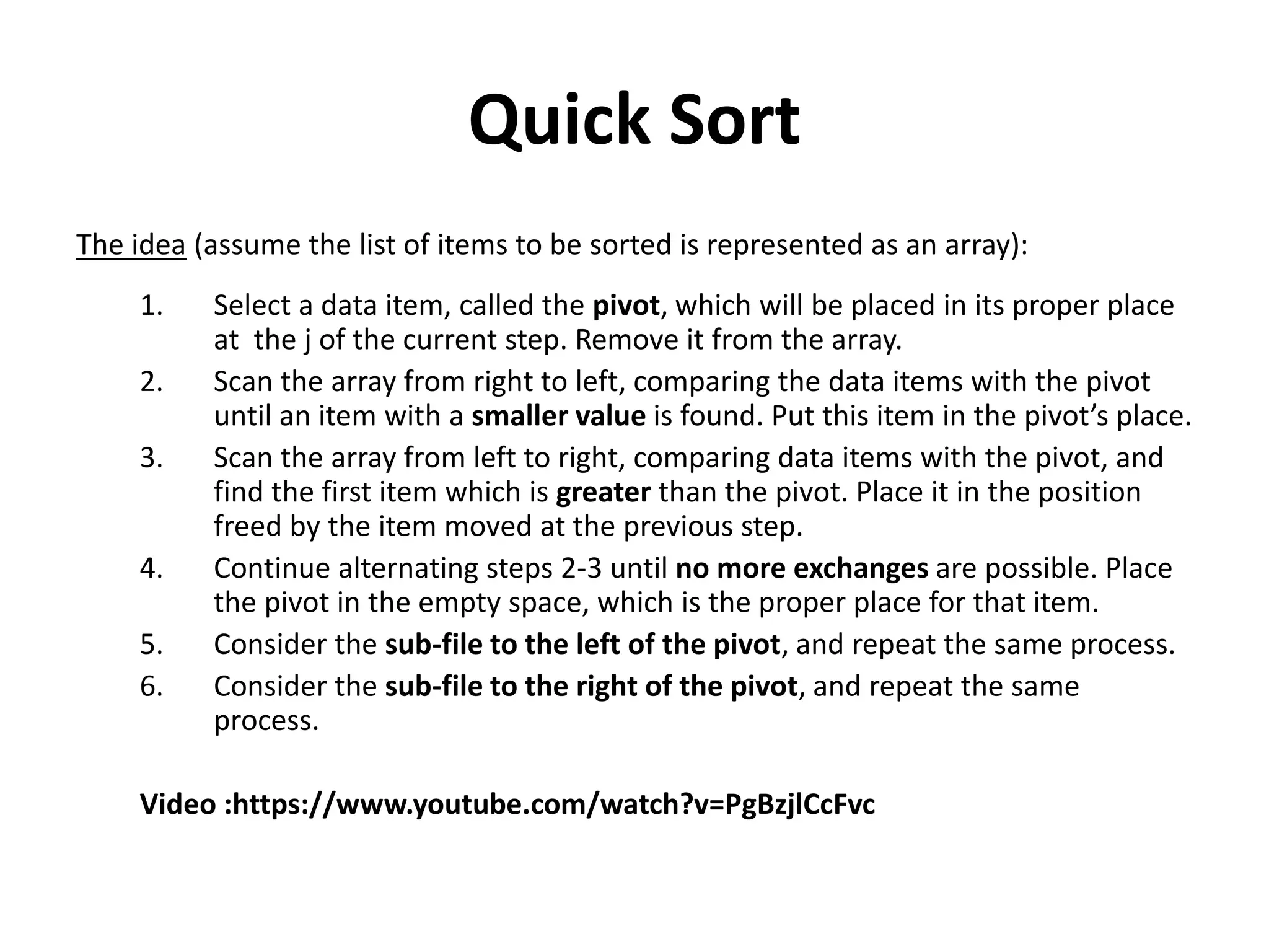
Quick Sort
The idea(assume the list of items to be sorted is represented as an array):
1. Select a data item, called the pivot, which will be placed in its proper place
at the j of the current step. Remove it from the array.
2. Scan the array from right to left, comparing the data items with the pivot
until an item with a smaller value is found. Put this item in the pivot’s place.
3. Scan the array from left to right, comparing data items with the pivot, and
find the first item which is greater than the pivot. Place it in the position
freed by the item moved at the previous step.
4. Continue alternating steps 2-3 until no more exchanges are possible. Place
the pivot in the empty space, which is the proper place for that item.
5. Consider the sub-file to the left of the pivot, and repeat the same process.
6. Consider the sub-file to the right of the pivot, and repeat the same
process.
Video :https://www.youtube.com/watch?v=PgBzjlCcFvc
17.
Example
We are givenarray of n integers to sort:
40 20 10 80 60 50 7 30 100
[0] [1] [2] [3] [4] [5] [6] [7] [8]
18.
Pick Pivot Element
Thereare a number of ways to pick the pivot element. In
this example, we will use the first element in the array:
40 20 10 80 60 50 7 30 100
[0] [1] [2] [3] [4] [5] [6] [7] [8]
40 20 1080 60 50 7 30 100pivot_index = 0
[0] [1] [2] [3] [4] [5] [6] [7] [8]
i j
1. While data[i] <= data[pivot]
++ i
21.
40 20 1080 60 50 7 30 100pivot_index = 0
i j
1. While data[i] <= data[pivot]
++ i
[0] [1] [2] [3] [4] [5] [6] [7] [8]
22.
40 20 1080 60 50 7 30 100pivot_index = 0
i j
1. While data[i] <= data[pivot]
++ i
[0] [1] [2] [3] [4] [5] [6] [7] [8]
23.
40 20 1080 60 50 7 30 100pivot_index = 0
i j
1. While data[i] <= data[pivot]
++ i
2. While data[j] > data[pivot]
--j
[0] [1] [2] [3] [4] [5] [6] [7] [8]
24.
40 20 1080 60 50 7 30 100pivot_index = 0
i j
1. While data[i] <= data[pivot]
++ i
2. While data[j] > data[pivot]
--j
[0] [1] [2] [3] [4] [5] [6] [7] [8]
25.
40 20 1080 60 50 7 30 100pivot_index = 0
i j
1. While data[i] <= data[pivot]
++ i
2. While data[j] > data[pivot]
--j
3. If i > j
swap data[i] and data[j]
[0] [1] [2] [3] [4] [5] [6] [7] [8]
26.
40 20 1030 60 50 7 80 100pivot_index = 0
i j
1. While data[i] <= data[pivot]
++ i
2. While data[j] > data[pivot]
--j
3. If i > j
swap data[i] and data[j]
[0] [1] [2] [3] [4] [5] [6] [7] [8]
27.
40 20 1030 60 50 7 80 100pivot_index = 0
i j
1. While data[i] <= data[pivot]
++ i
2. While data[j] > data[pivot]
--j
3. If i > j
swap data[i] and data[j]
4. While j > i, go to 1.
[0] [1] [2] [3] [4] [5] [6] [7] [8]
28.
40 20 1030 60 50 7 80 100pivot_index = 0
i j
1. While data[i] <= data[pivot]
++ i
2. While data[j] > data[pivot]
--j
3. If i > j
swap data[i] and data[j]
4. While j> i, go to 1.
[0] [1] [2] [3] [4] [5] [6] [7] [8]
29.
40 20 1030 60 50 7 80 100pivot_index = 0
i j
1. While data[i] <= data[pivot]
++ i
2. While data[j] > data[pivot]
--j
3. If i > j
swap data[i] and [j]
4. While j> i, go to 1.
[0] [1] [2] [3] [4] [5] [6] [7] [8]
30.
40 20 1030 60 50 7 80 100pivot_index = 0
i j
1. While data[i] <= data[pivot]
++ i
2. While data[j] > data[pivot]
--j
3. If i > j
swap data[i] and data[j]
4. While j> i, go to 1.
[0] [1] [2] [3] [4] [5] [6] [7] [8]
31.
40 20 1030 60 50 7 80 100pivot_index = 0
i j
1. While data[i] <= data[pivot]
++ i
2. While data[j] > data[pivot]
--j
3. If i > j
swap data[i] and data[j]
4. While j > i, go to 1.
[0] [1] [2] [3] [4] [5] [6] [7] [8]
32.
40 20 1030 60 50 7 80 100pivot_index = 0
i j
1. While data[i] <= data[pivot]
++ i
2. While data[j] > data[pivot]
--j
3. If i > j
swap data[i] and data[j]
4. While j > i, go to 1.
[0] [1] [2] [3] [4] [5] [6] [7] [8]
33.
1. While data[i]<= data[pivot]
++ i
2. While data[j] > data[pivot]
--j
3. If i > j
swap data[i] and data[j]
4. While j > i, go to 1.
40 20 10 30 7 50 60 80 100pivot_index = 0
i j
[0] [1] [2] [3] [4] [5] [6] [7] [8]
34.
1. While data[i]<= data[pivot]
++i
2. While data[j] > data[pivot]
--j
3. If i > j
swap data[i] and data[j]
4. While j > i, go to 1.
40 20 10 30 7 50 60 80 100pivot_index = 0
i j
[0] [1] [2] [3] [4] [5] [6] [7] [8]
35.
1. While data[i]<= data[pivot]
++i
2. While data[j] > data[pivot]
--j
3. If i > j
swap data[i] and data[j]
4. While j > i, go to 1.
40 20 10 30 7 50 60 80 100pivot_index = 0
i j
[0] [1] [2] [3] [4] [5] [6] [7] [8]
36.
1. While data[i]<= data[pivot]
++i
2. While data[j] > data[pivot]
--j
3. If i > j
swap data[i] and data[j]
4. While j > i, go to 1.
40 20 10 30 7 50 60 80 100pivot_index = 0
i j
[0] [1] [2] [3] [4] [5] [6] [7] [8]
37.
1. While data[i]<= data[pivot]
++i
2. While data[j] > data[pivot]
--j
3. If i > j
swap data[i] and data[j]
4. While j > i, go to 1.
40 20 10 30 7 50 60 80 100pivot_index = 0
i j
[0] [1] [2] [3] [4] [5] [6] [7] [8]
38.
1. While data[i]<= data[pivot]
++i
2. While data[j] > data[pivot]
--j
3. If i > j
swap data[i] and data[j]
4. While j > i, go to 1.
40 20 10 30 7 50 60 80 100pivot_index = 0
i j
[0] [1] [2] [3] [4] [5] [6] [7] [8]
39.
1. While data[i]<= data[pivot]
++i
2. While data[j] > data[pivot]
--j
3. If i > j
swap data[i] and data[j]
4. While j > i, go to 1.
40 20 10 30 7 50 60 80 100pivot_index = 0
i j
[0] [1] [2] [3] [4] [5] [6] [7] [8]
40.
1. While data[i]<= data[pivot]
++i
2. While data[j] > data[pivot]
--j
3. If i > j
swap data[i] and data[j]
4. While j > i, go to 1.
40 20 10 30 7 50 60 80 100pivot_index = 0
i j
[0] [1] [2] [3] [4] [5] [6] [7] [8]
41.
1. While data[i]<= data[pivot]
++i
2. While data[j] > data[pivot]
--j
3. If i > j
swap data[i] and data[j]
4. While j > i, go to 1.
40 20 10 30 7 50 60 80 100pivot_index = 0
i j
[0] [1] [2] [3] [4] [5] [6] [7] [8]
42.
1. While data[i]<= data[pivot]
++i
2. While data[j] > data[pivot]
--j
3. If i > j
swap data[i] and data[j]
4. While j > i, go to 1.
5. Swap data[j] and data[pivot_index]
40 20 10 30 7 50 60 80 100pivot_index = 0
i j
[0] [1] [2] [3] [4] [5] [6] [7] [8]
43.
1. While data[i]<= data[pivot]
++i
2. While data[j] > data[pivot]
--j
3. If i > j
swap data[i] and data[j]
4. While j > i, go to 1.
5. Swap data[j] and data[pivot_index]
7 20 10 30 40 50 60 80 100pivot_index = 4
i j
[0] [1] [2] [3] [4] [5] [6] [7] [8]
Quick Sort Algorithm
InQuick sort algorithm, partitioning of the list is performed using
following steps...
Step 1 - Consider the first element of the list as pivot (i.e., Element at
first position in the list).
Step 2 - Define two variables i and j. Set i and j to first and last elements
of the list respectively.
Step 3 - Increment i until list[i] > pivot then stop.
Step 4 - Decrement j until list[j] < pivot then stop.
Step 5 - If i > j then exchange list[i] and list[j].
Step 6 - Repeat steps 3,4 & 5 until I < j.
Step 7 - Exchange the pivot element with list[j] element.
46.
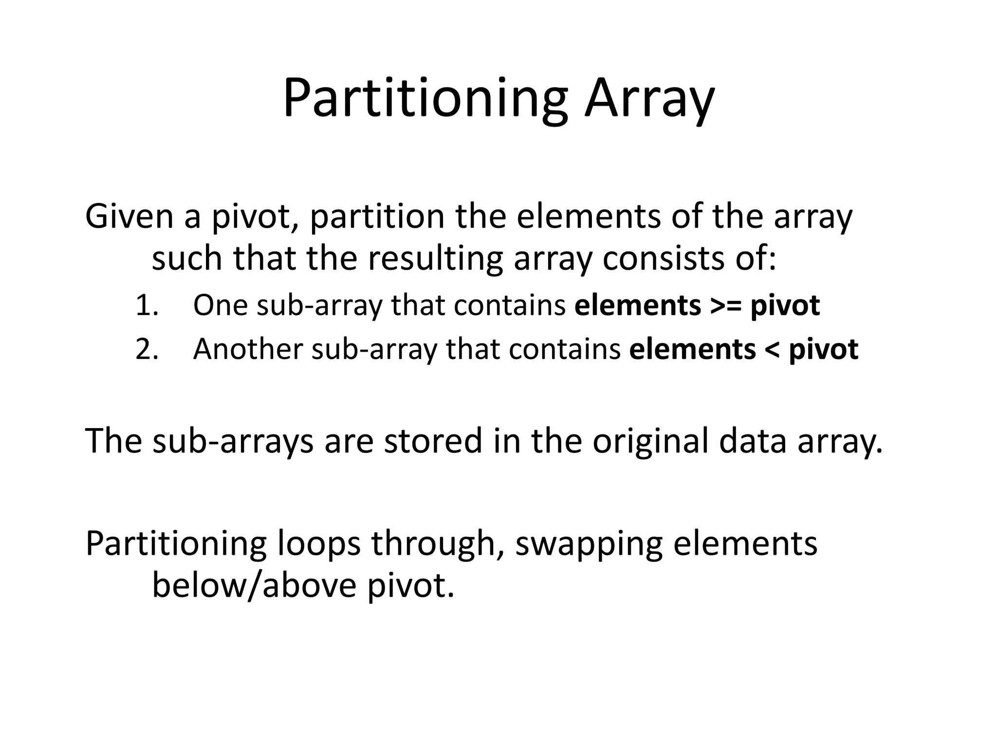
Partitioning Array
Given apivot, partition the elements of the array
such that the resulting array consists of:
1. One sub-array that contains elements >= pivot
2. Another sub-array that contains elements < pivot
The sub-arrays are stored in the original data array.
Partitioning loops through, swapping elements
below/above pivot.
47.
Quick Sort
40 2010 80 60 50 7 30 100
[0] [1] [2] [3] [4] [5] [6] [7] [8]
m n
K = Pivot
Ki
Kj
i
j
m nj-1
j
j+1
48.
CHAPTER 7 48
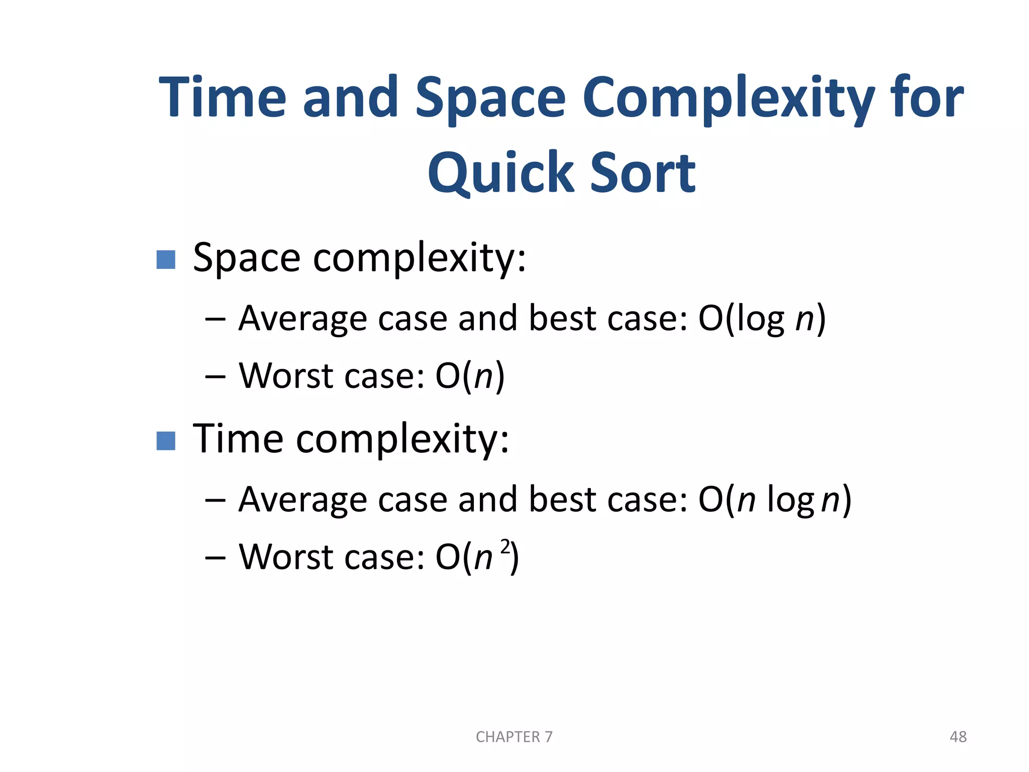
Timeand Space Complexity for
Quick Sort
Space complexity:
– Average case and best case: O(log n)
– Worst case: O(n)
Time complexity:
– Average case and best case: O(n logn)
– Worst case: O(n )2
49.
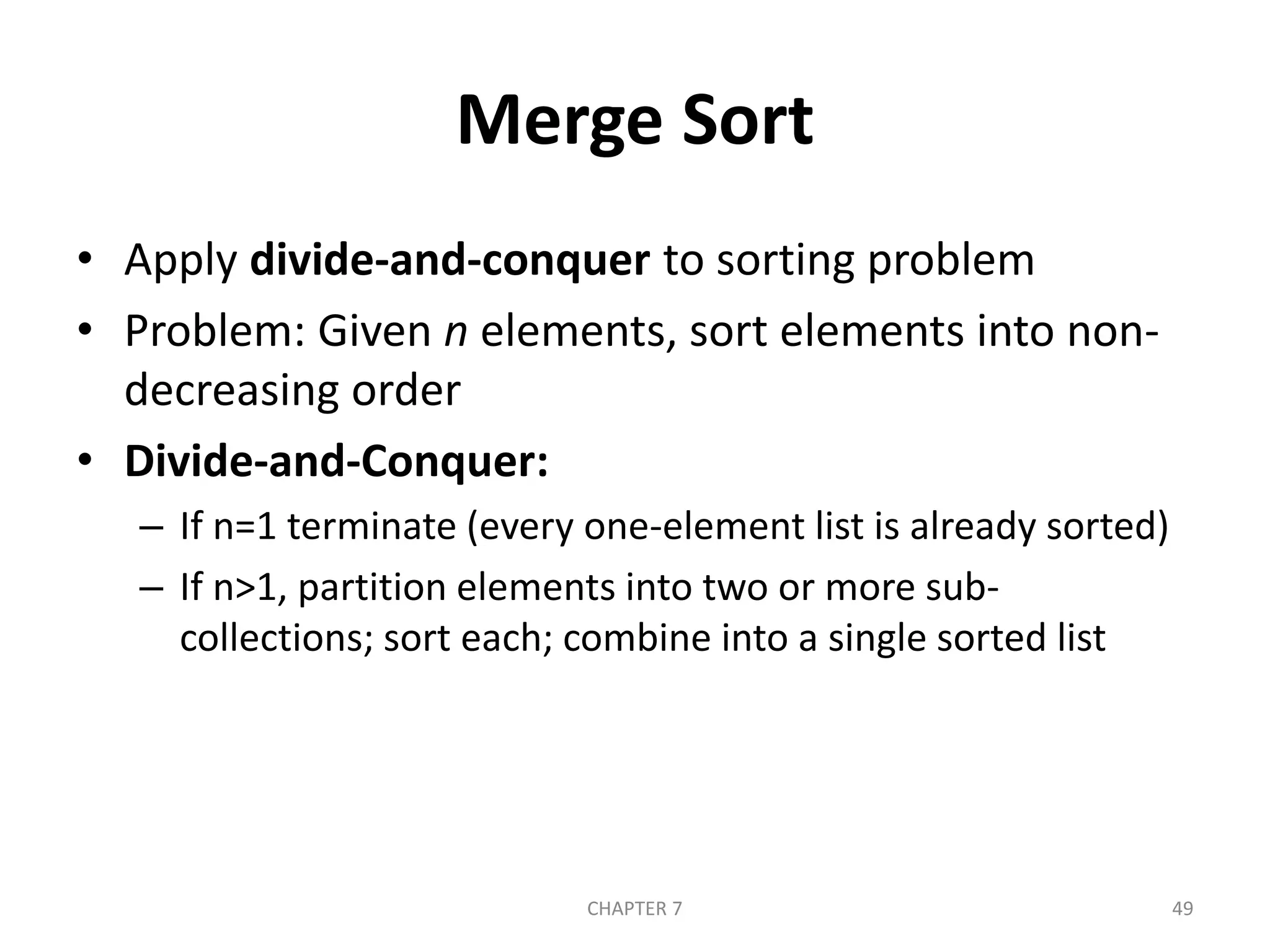
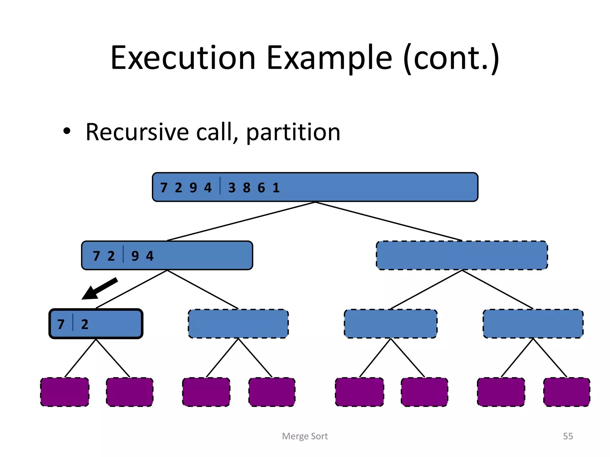
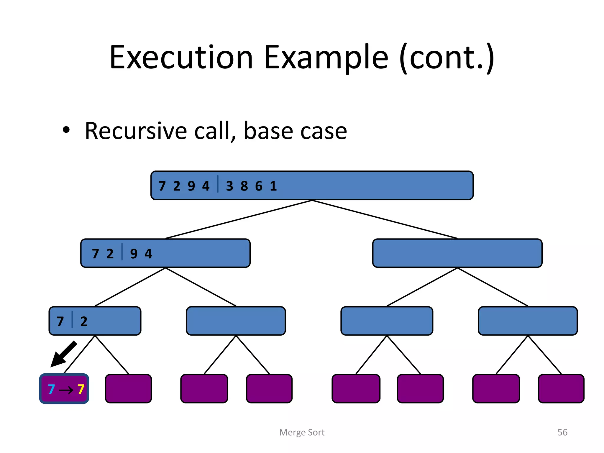
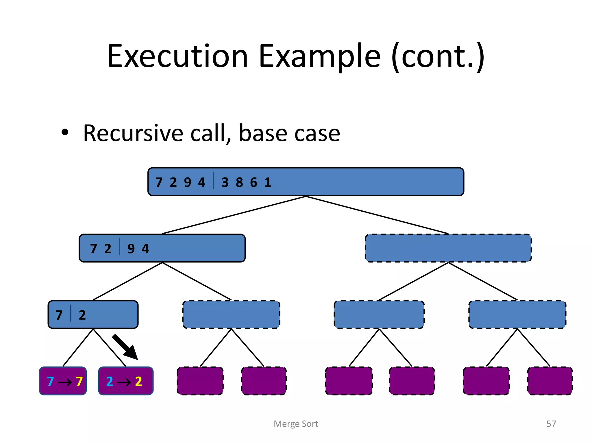
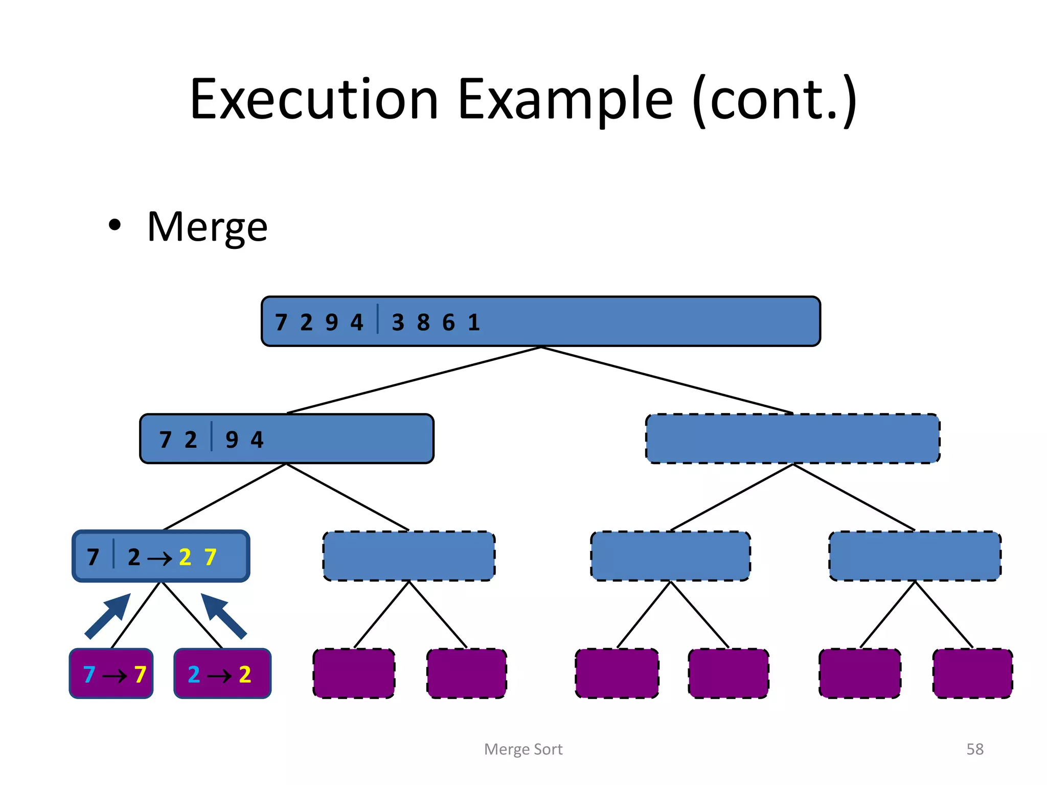
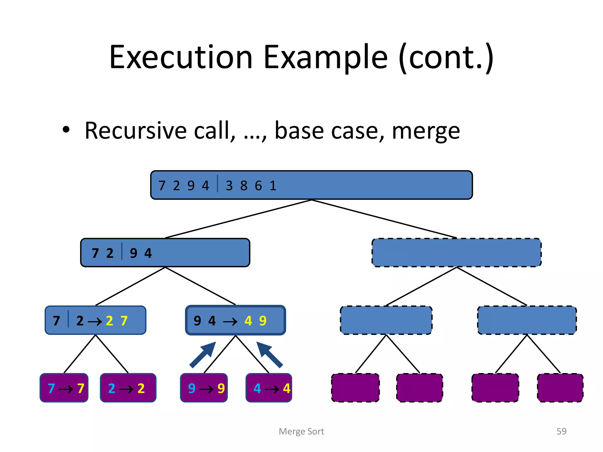
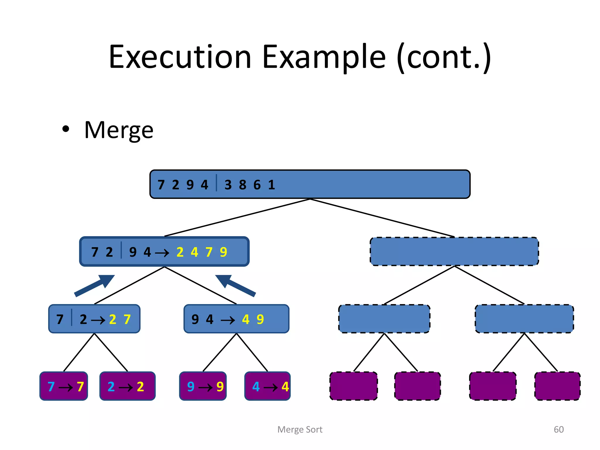
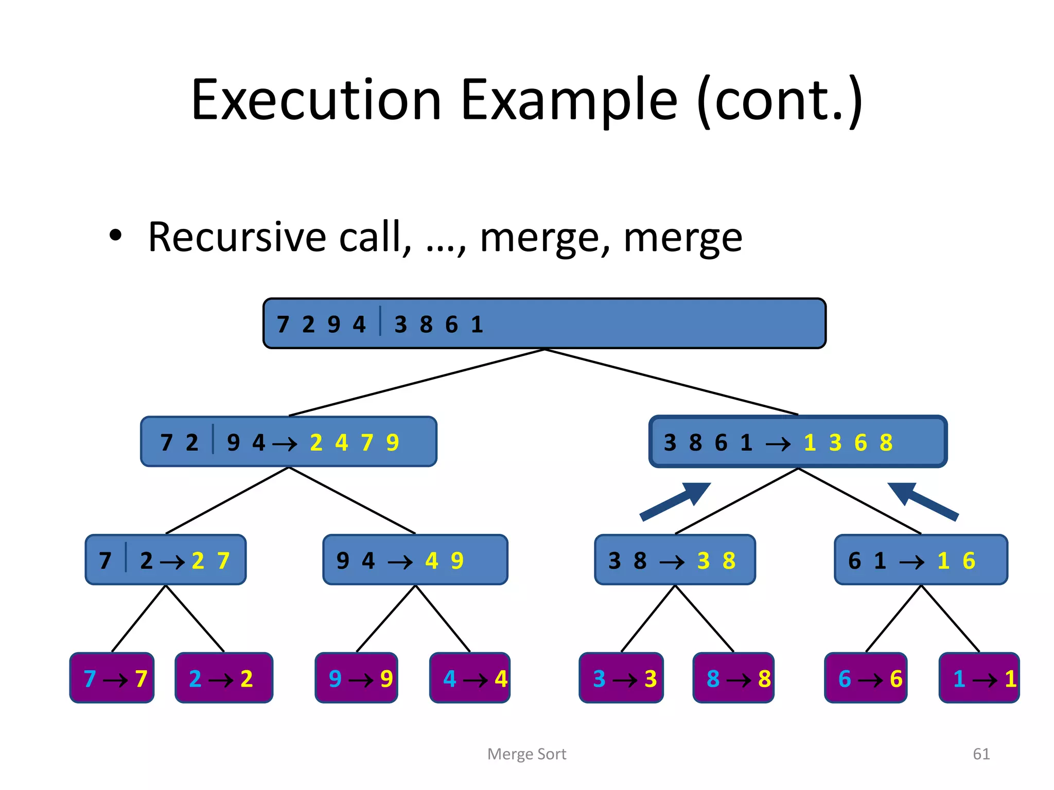
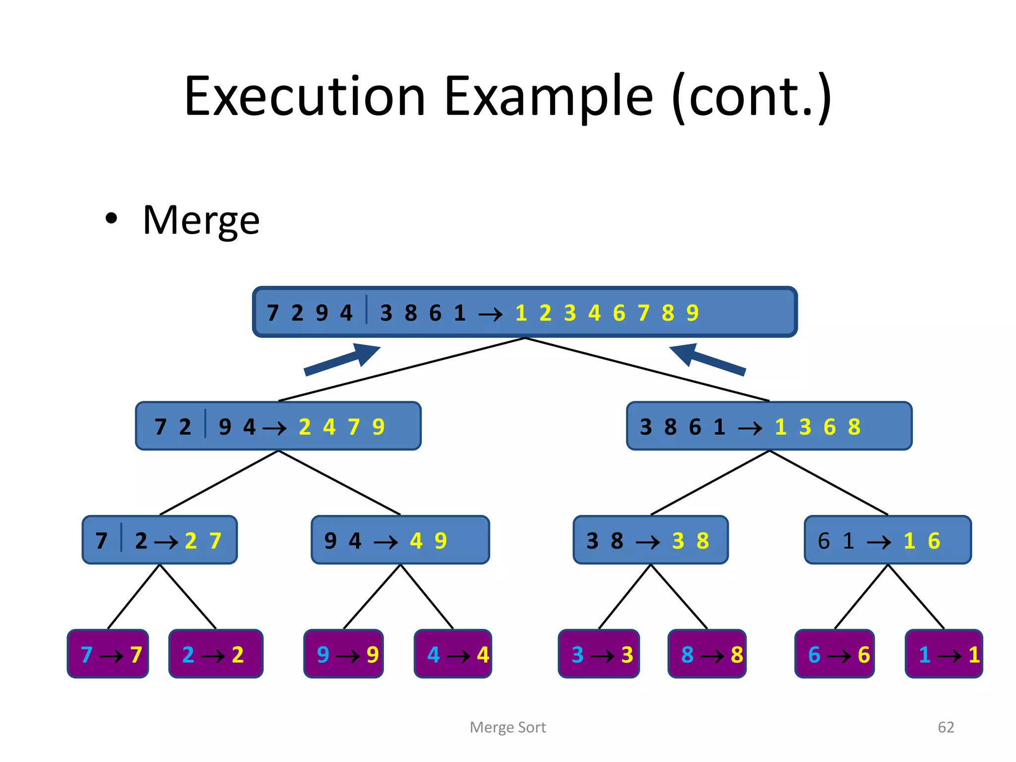
Merge Sort
• Applydivide-and-conquer to sorting problem
• Problem: Given n elements, sort elements into non-
decreasing order
• Divide-and-Conquer:
– If n=1 terminate (every one-element list is already sorted)
– If n>1, partition elements into two or more sub-
collections; sort each; combine into a single sorted list
CHAPTER 7 49
50.
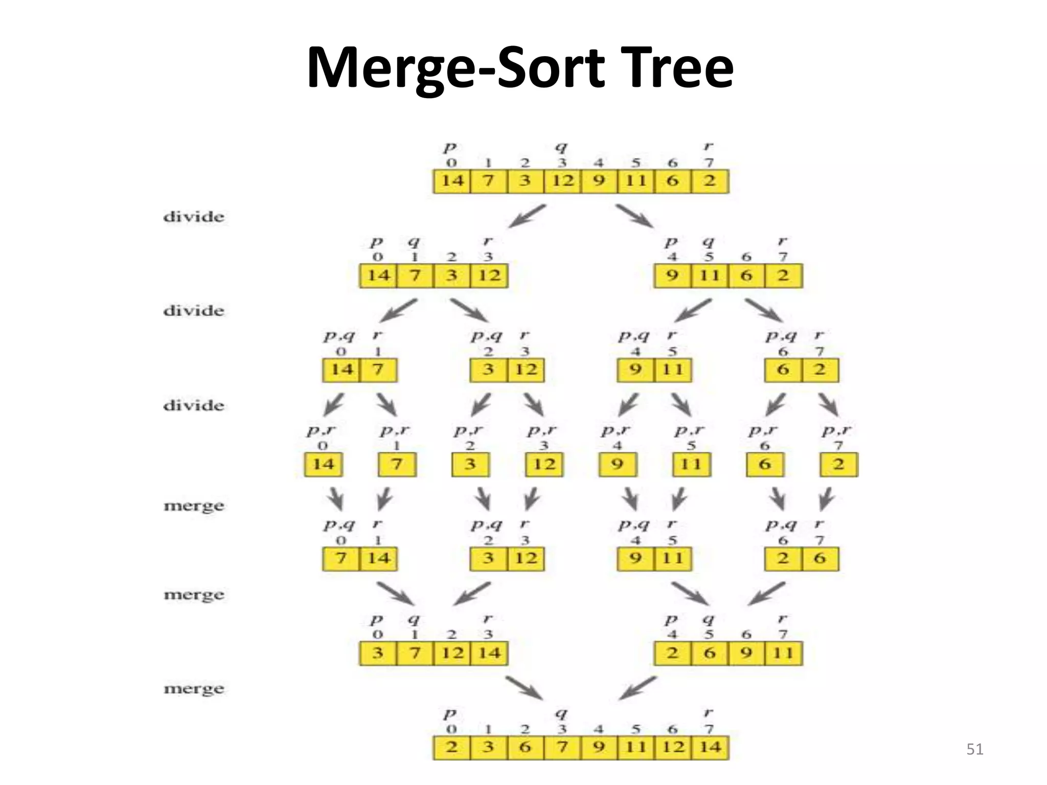
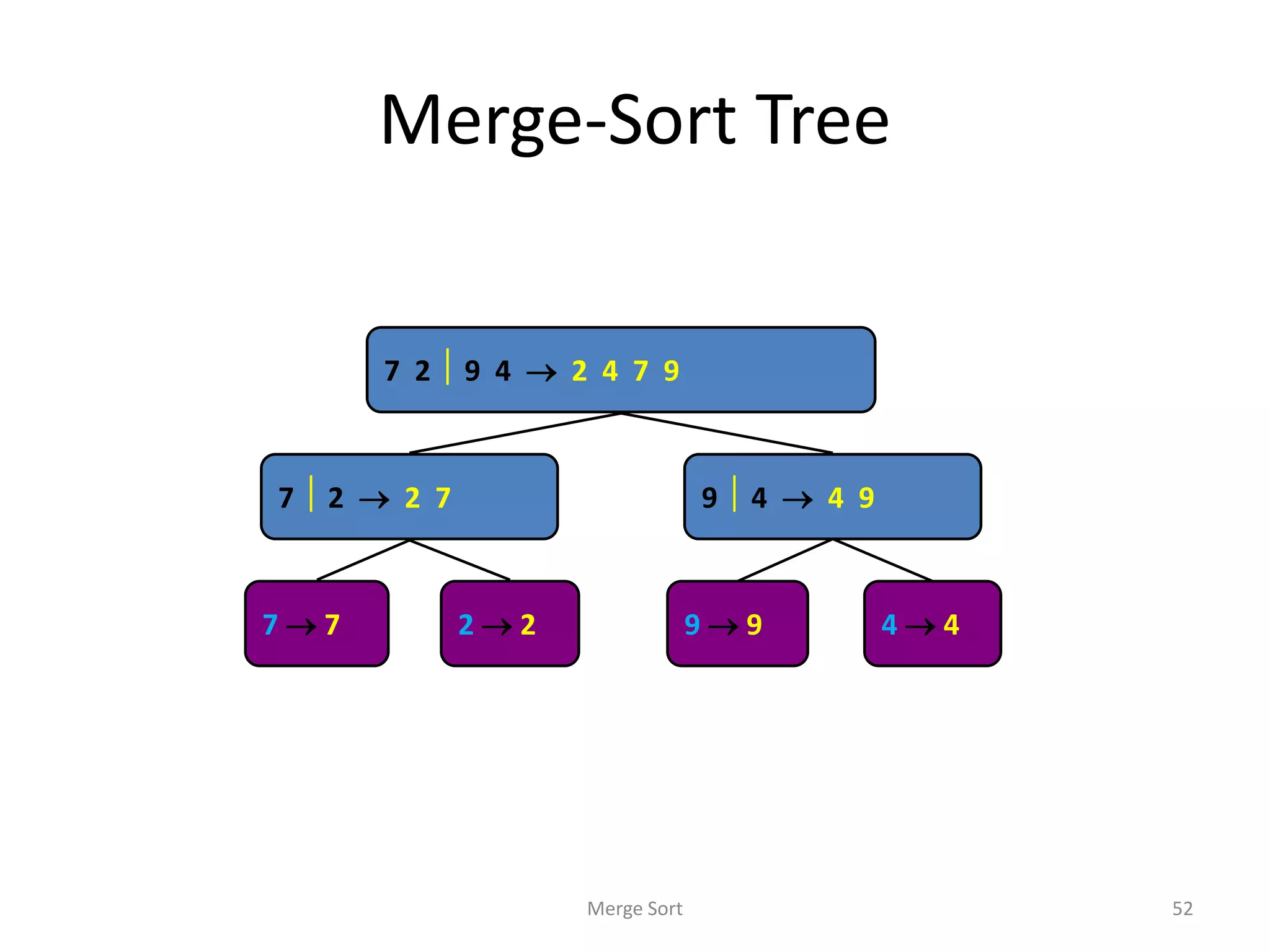
Merge-Sort
• An executionof merge-sort is depicted by a binary
tree
– each node represents a recursive call of merge-sort and
stores
– the root is the initial call
– the leaves are calls on subsequences of size 0 or 1
• Given two sorted lists
(list[i], …, list[m])
(list[m+1], …, list[n])
generate a single sorted list
(sorted[i], …, sorted[n])
• O(n) space vs. O(1) space
Merge Sort 50
Merge Sort
[3, 4,6, 10]
[2, 3, 4, 5, 6, 7, 8, 10 ]
[2, 5, 7, 8]
[10, 4, 6, 3, 8, 2, 5, 7]Input Array
Output Array (Sorted)
X X
K
Xi Xj
Zk
66.
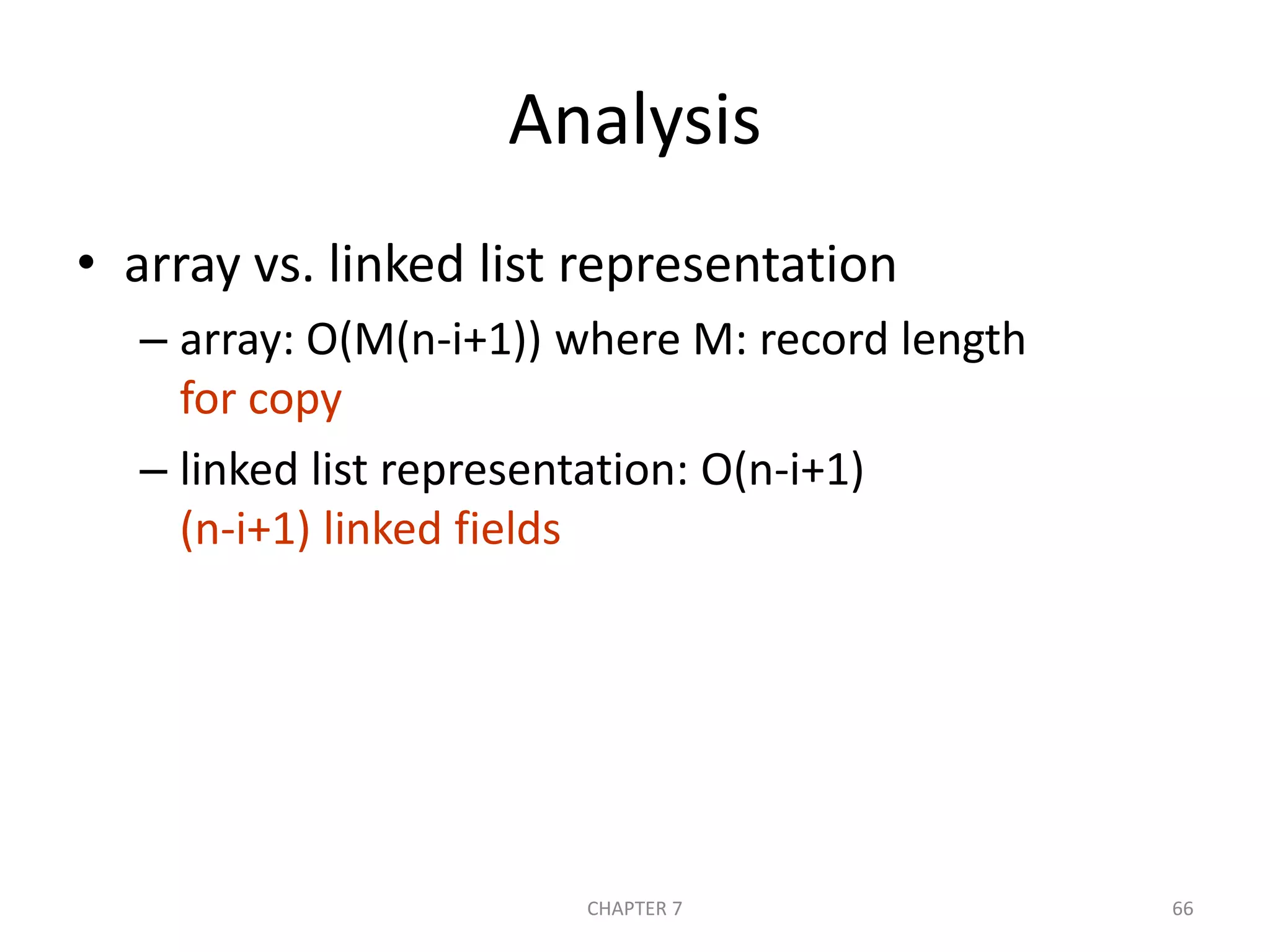
Analysis
• array vs.linked list representation
– array: O(M(n-i+1)) where M: record length
for copy
– linked list representation: O(n-i+1)
(n-i+1) linked fields
CHAPTER 7 66
67.
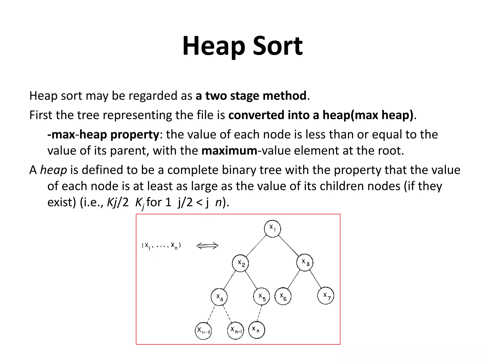
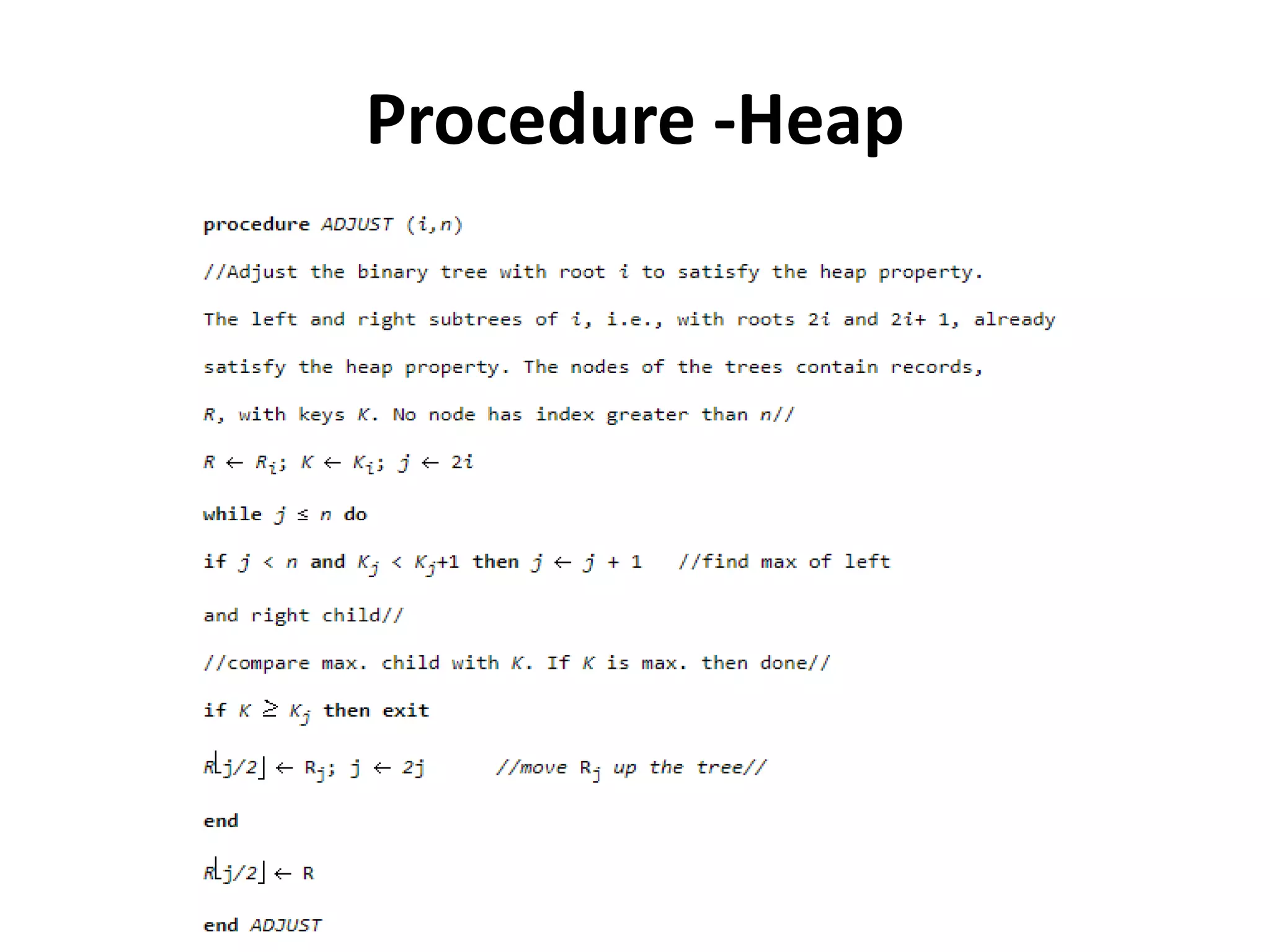
Heap Sort
Heap sortmay be regarded as a two stage method.
First the tree representing the file is converted into a heap(max heap).
-max-heap property: the value of each node is less than or equal to the
value of its parent, with the maximum-value element at the root.
A heap is defined to be a complete binary tree with the property that the value
of each node is at least as large as the value of its children nodes (if they
exist) (i.e., Kj/2 Kj for 1 j/2 < j n).
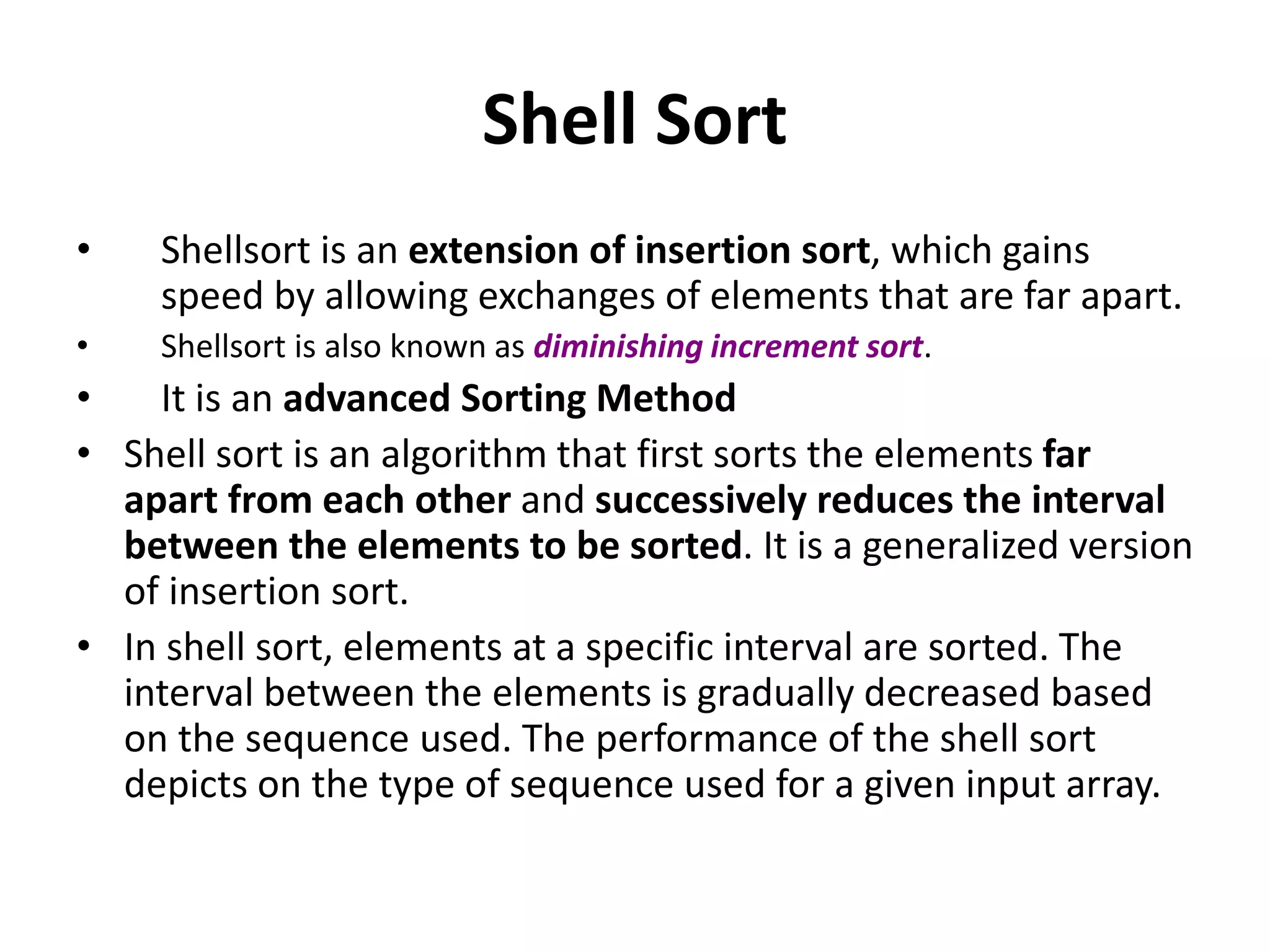
Shell Sort
• Shellsortis an extension of insertion sort, which gains
speed by allowing exchanges of elements that are far apart.
• Shellsort is also known as diminishing increment sort.
• It is an advanced Sorting Method
• Shell sort is an algorithm that first sorts the elements far
apart from each other and successively reduces the interval
between the elements to be sorted. It is a generalized version
of insertion sort.
• In shell sort, elements at a specific interval are sorted. The
interval between the elements is gradually decreased based
on the sequence used. The performance of the shell sort
depicts on the type of sequence used for a given input array.
75.
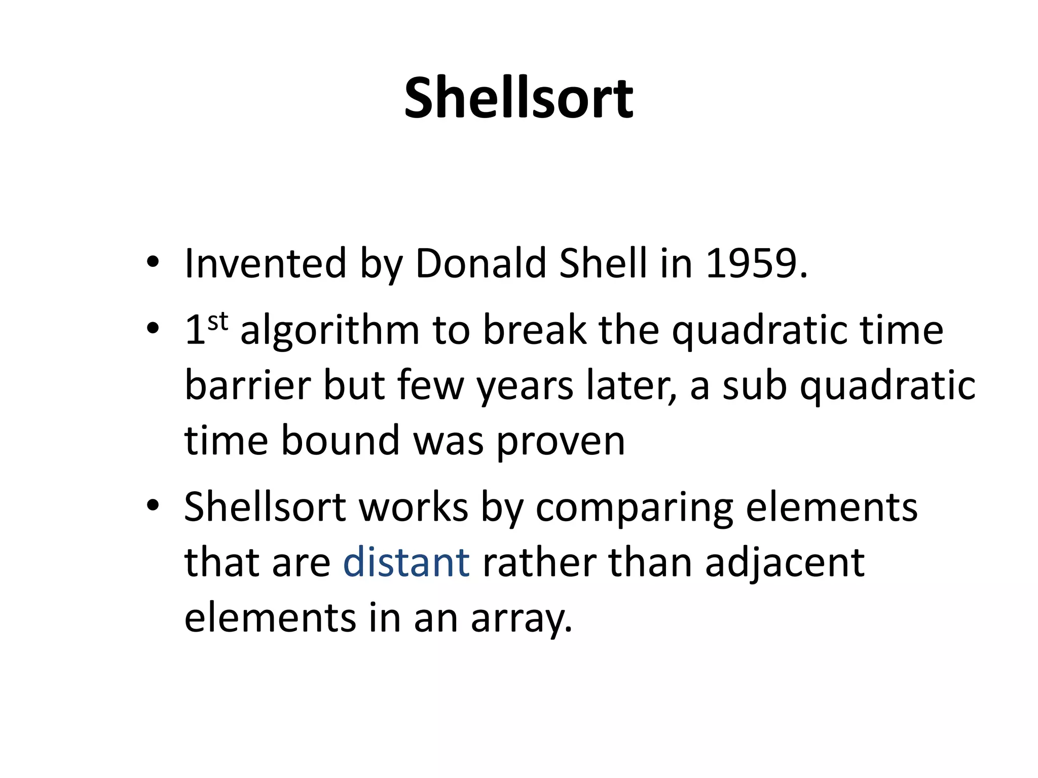
Shellsort
• Invented byDonald Shell in 1959.
• 1st algorithm to break the quadratic time
barrier but few years later, a sub quadratic
time bound was proven
• Shellsort works by comparing elements
that are distant rather than adjacent
elements in an array.
76.
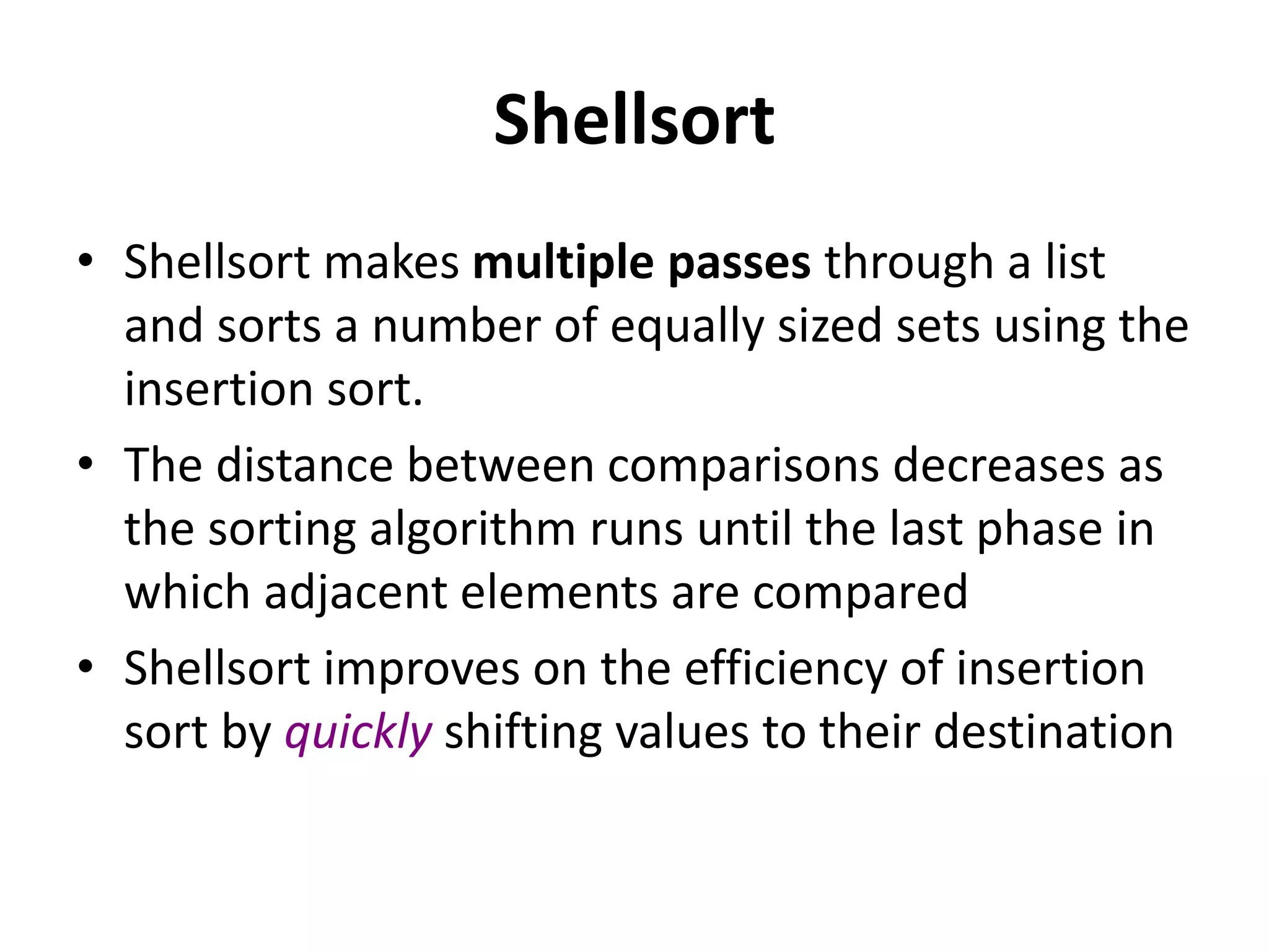
Shellsort
• Shellsort makesmultiple passes through a list
and sorts a number of equally sized sets using the
insertion sort.
• The distance between comparisons decreases as
the sorting algorithm runs until the last phase in
which adjacent elements are compared
• Shellsort improves on the efficiency of insertion
sort by quickly shifting values to their destination
77.
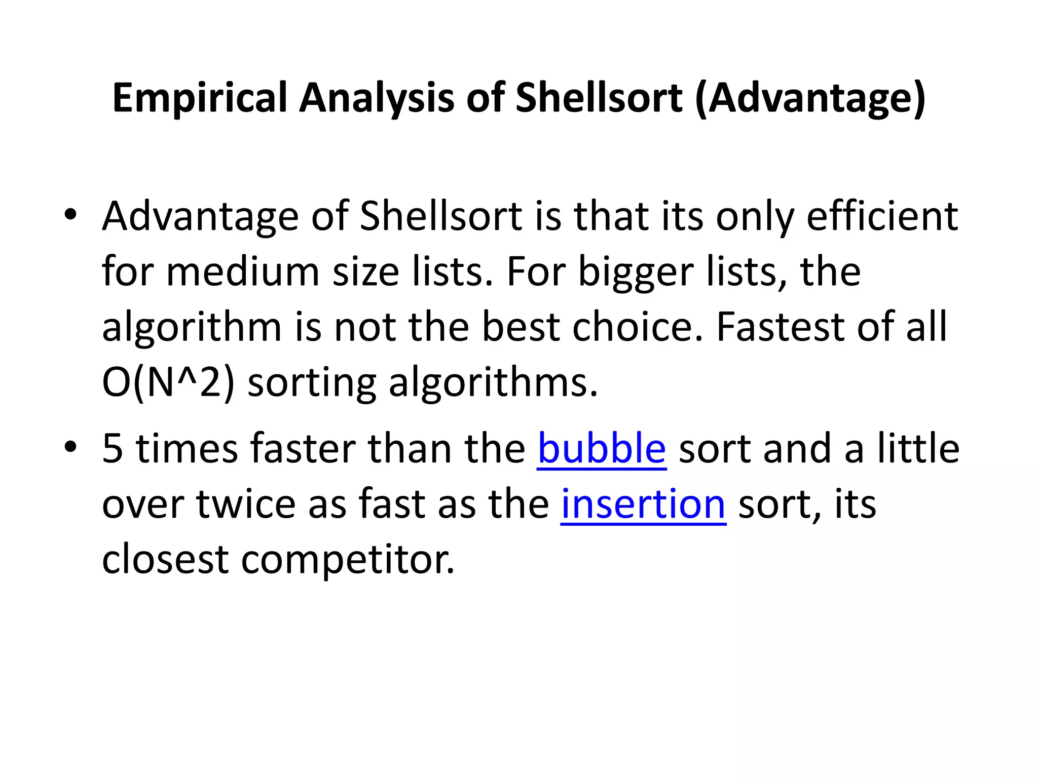
Empirical Analysis ofShellsort (Advantage)
• Advantage of Shellsort is that its only efficient
for medium size lists. For bigger lists, the
algorithm is not the best choice. Fastest of all
O(N^2) sorting algorithms.
• 5 times faster than the bubble sort and a little
over twice as fast as the insertion sort, its
closest competitor.
78.
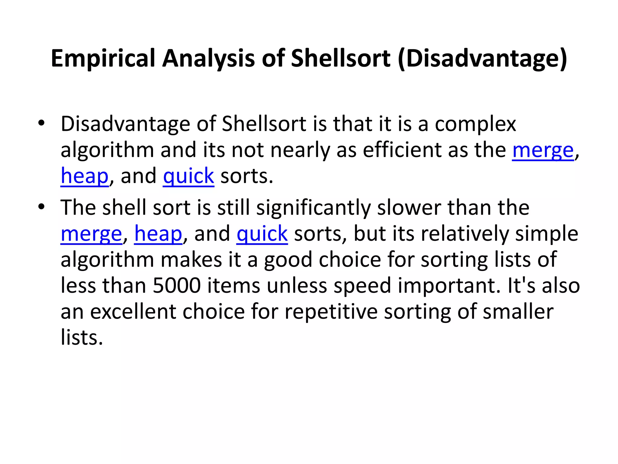
Empirical Analysis ofShellsort (Disadvantage)
• Disadvantage of Shellsort is that it is a complex
algorithm and its not nearly as efficient as the merge,
heap, and quick sorts.
• The shell sort is still significantly slower than the
merge, heap, and quick sorts, but its relatively simple
algorithm makes it a good choice for sorting lists of
less than 5000 items unless speed important. It's also
an excellent choice for repetitive sorting of smaller
lists.
79.
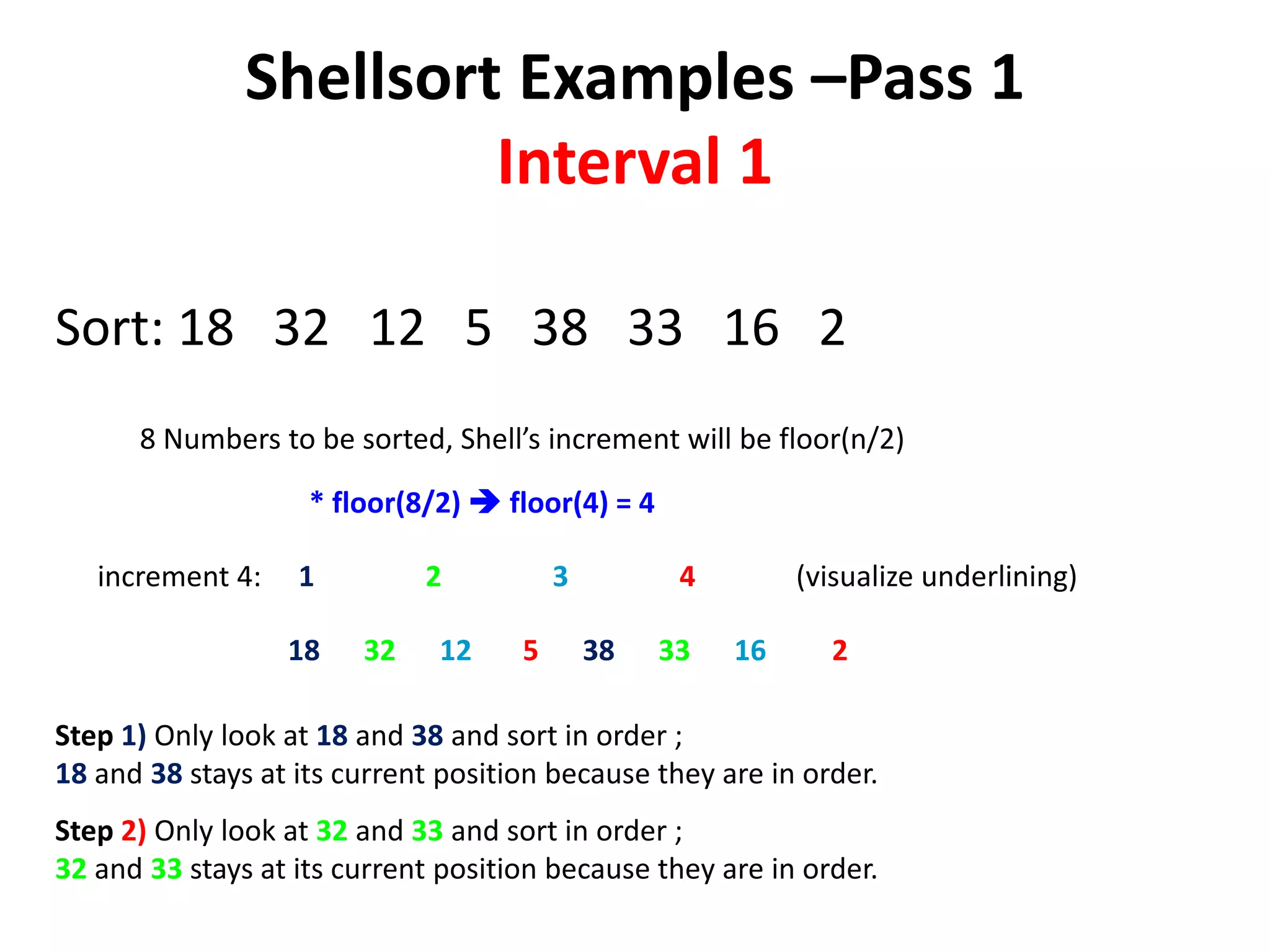
Shellsort Examples –Pass1
Interval 1
Sort: 18 32 12 5 38 33 16 2
8 Numbers to be sorted, Shell’s increment will be floor(n/2)
* floor(8/2) floor(4) = 4
increment 4: 1 2 3 4
18 32 12 5 38 33 16 2
(visualize underlining)
Step 1) Only look at 18 and 38 and sort in order ;
18 and 38 stays at its current position because they are in order.
Step 2) Only look at 32 and 33 and sort in order ;
32 and 33 stays at its current position because they are in order.
80.
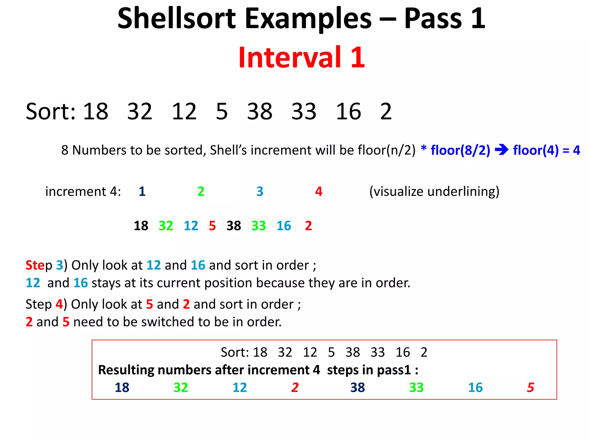
Shellsort Examples –Pass 1
Interval 1
Sort: 18 32 12 5 38 33 16 2
8 Numbers to be sorted, Shell’s increment will be floor(n/2) * floor(8/2) floor(4) = 4
increment 4: 1 2 3 4
18 32 12 5 38 33 16 2
(visualize underlining)
Step 3) Only look at 12 and 16 and sort in order ;
12 and 16 stays at its current position because they are in order.
Step 4) Only look at 5 and 2 and sort in order ;
2 and 5 need to be switched to be in order.
Sort: 18 32 12 5 38 33 16 2
Resulting numbers after increment 4 steps in pass1 :
18 32 12 2 38 33 16 5
81.
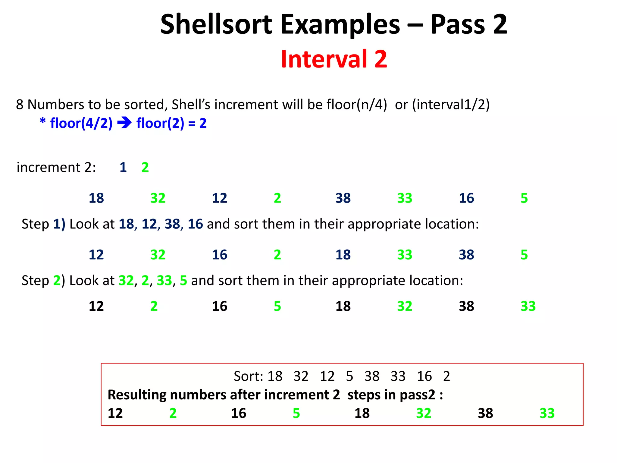
Shellsort Examples –Pass 2
Interval 2
8 Numbers to be sorted, Shell’s increment will be floor(n/4) or (interval1/2)
* floor(4/2) floor(2) = 2
increment 2: 1 2
18 32 12 2 38 33 16 5
Step 1) Look at 18, 12, 38, 16 and sort them in their appropriate location:
12 32 16 2 18 33 38 5
Step 2) Look at 32, 2, 33, 5 and sort them in their appropriate location:
12 2 16 5 18 32 38 33
Sort: 18 32 12 5 38 33 16 2
Resulting numbers after increment 2 steps in pass2 :
12 2 16 5 18 32 38 33
82.
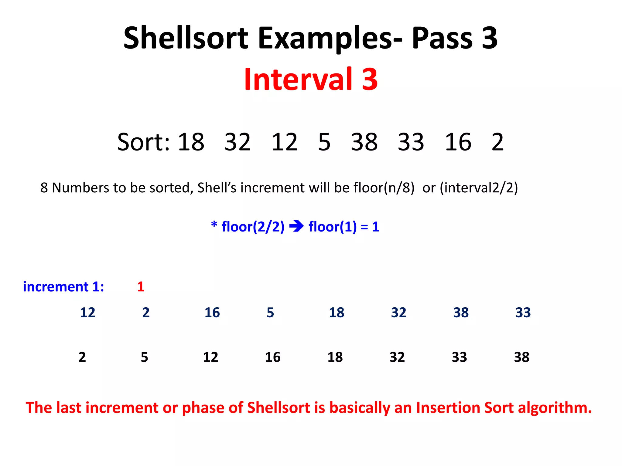
Shellsort Examples- Pass3
Interval 3
Sort: 18 32 12 5 38 33 16 2
* floor(2/2) floor(1) = 1
increment 1: 1
12 2 16 5 18 32 38 33
2 5 12 16 18 32 33 38
The last increment or phase of Shellsort is basically an Insertion Sort algorithm.
8 Numbers to be sorted, Shell’s increment will be floor(n/8) or (interval2/2)
83.
Shell Sort Algorithm
1.shellsort(intarr[], int num)
2.{
3.int i, j, k;
4.for (i = num / 2; i > 0; i = i / 2)
5.{
6.for (j = i; j < num; j++)
7.{
8.for(k = j - i; k >= 0; k = k - i)
9.{
10.if (arr[k+i] >= arr[k])
11.break;
12.else
13.{
14.Swap arr[k] =
arr[k+i];}
15.}
16.}
17.}
18.}
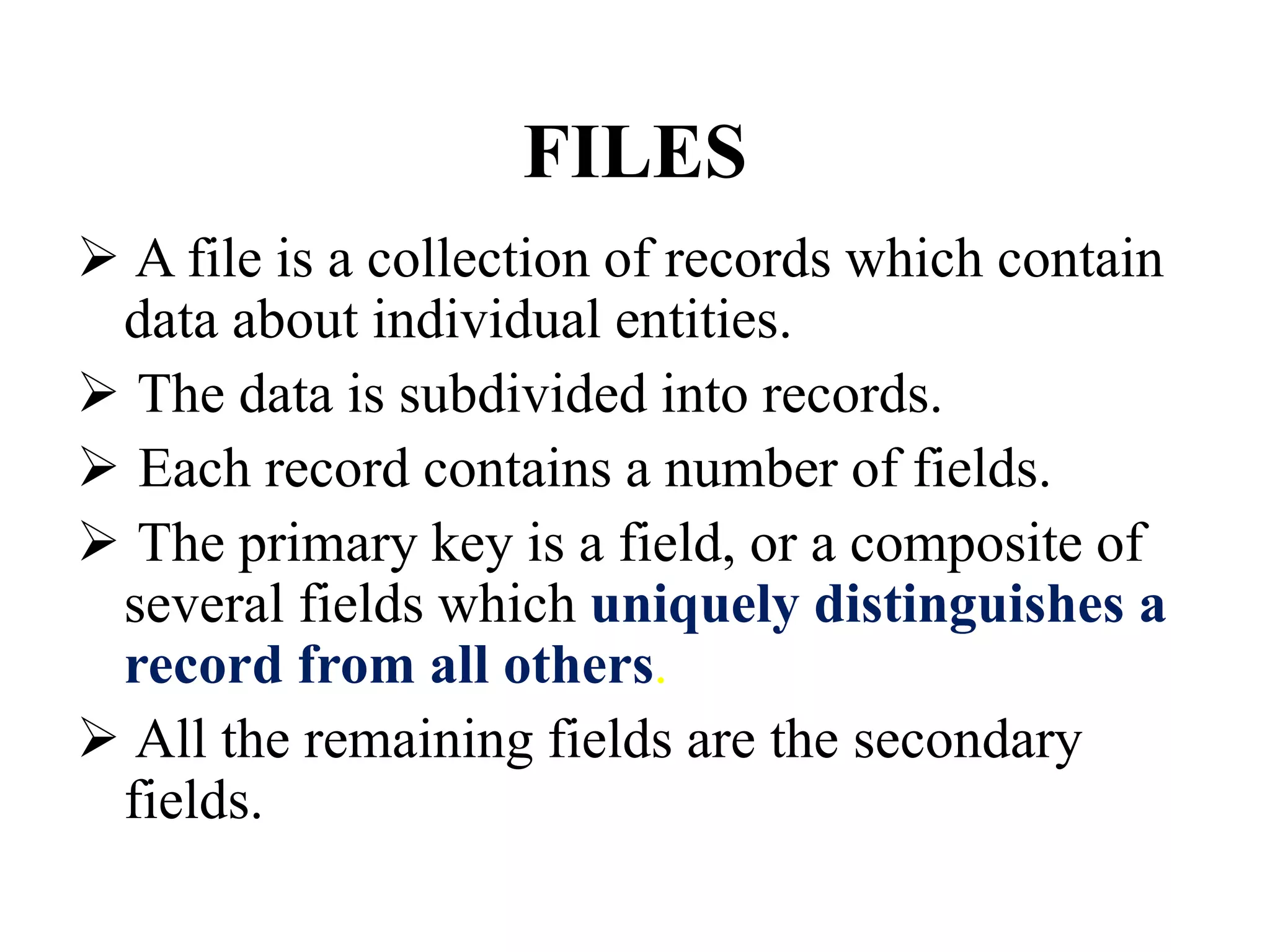
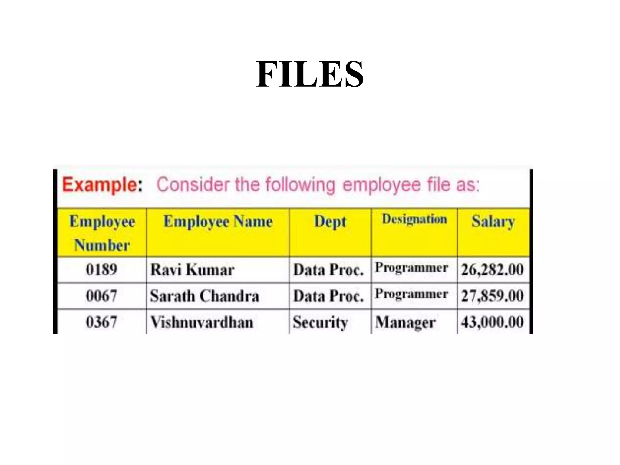
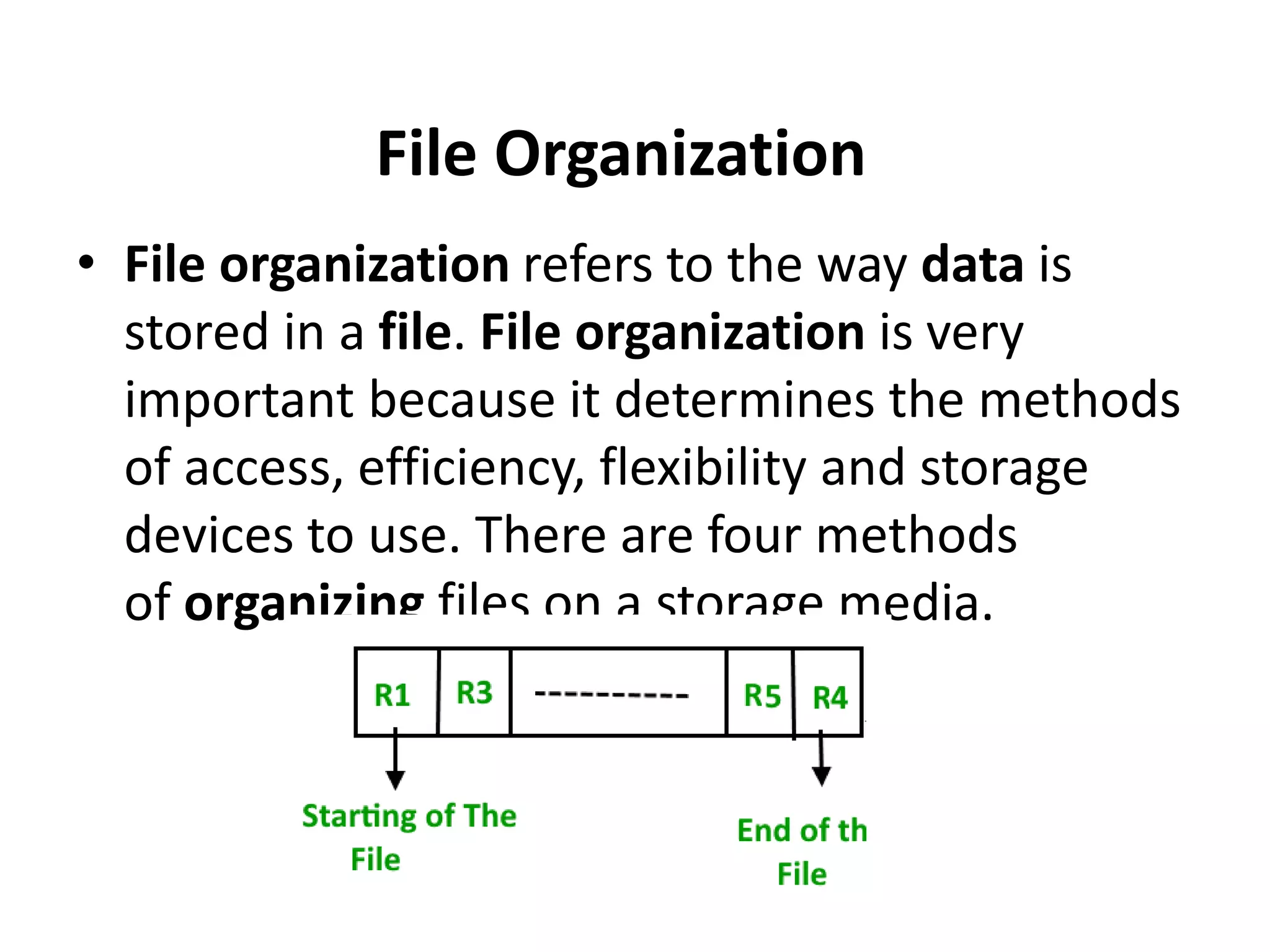
FILES
A fileis a collection of records which contain
data about individual entities.
The data is subdivided into records.
Each record contains a number of fields.
The primary key is a field, or a composite of
several fields which uniquely distinguishes a
record from all others.
All the remaining fields are the secondary
fields.
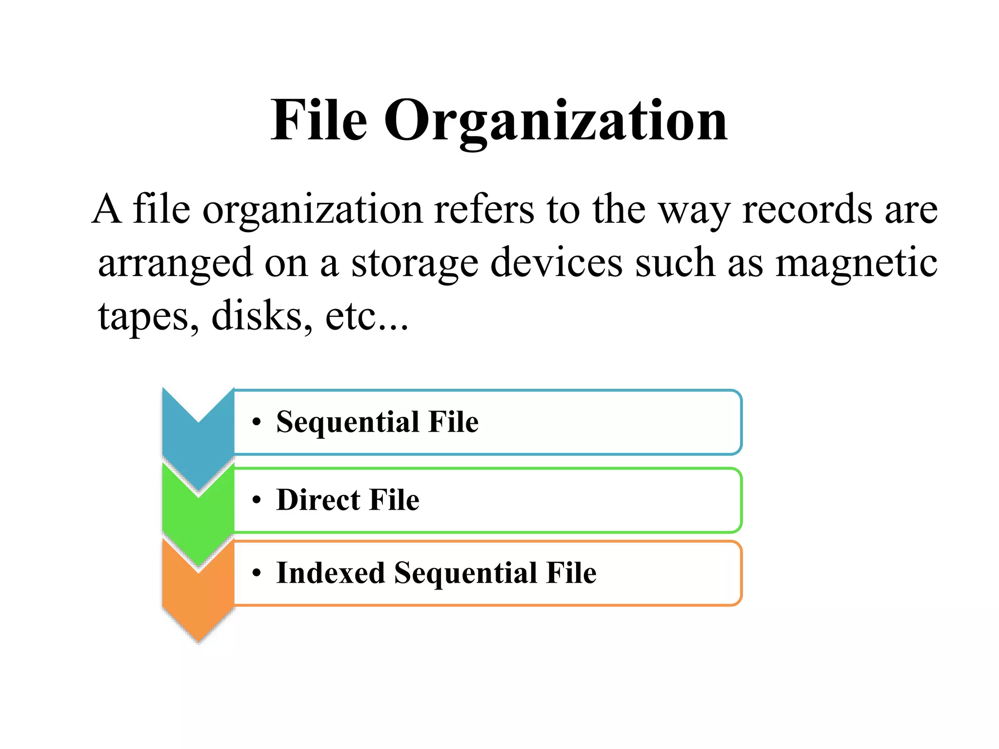
File Organization
A fileorganization refers to the way records are
arranged on a storage devices such as magnetic
tapes, disks, etc...
• Sequential File
• Direct File
• Indexed Sequential File
89.
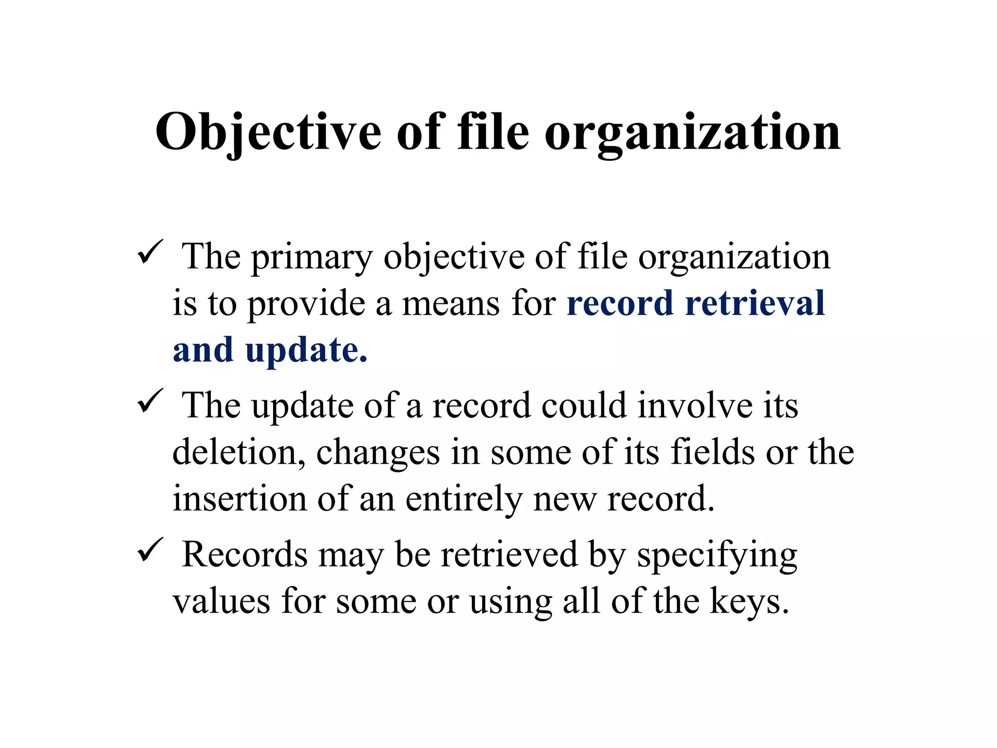
Objective of fileorganization
The primary objective of file organization
is to provide a means for record retrieval
and update.
The update of a record could involve its
deletion, changes in some of its fields or the
insertion of an entirely new record.
Records may be retrieved by specifying
values for some or using all of the keys.
90.
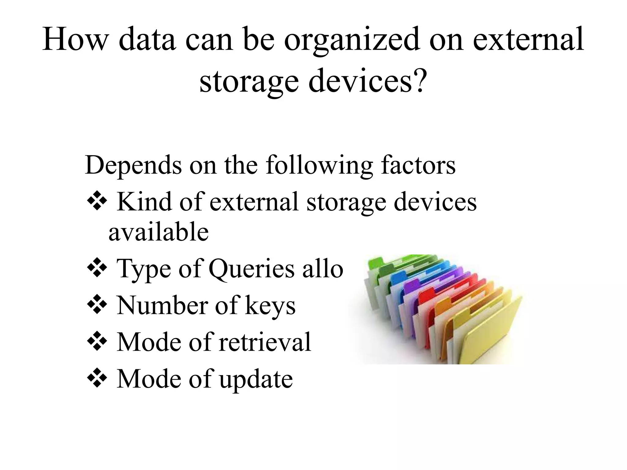
How data canbe organized on external
storage devices?
Depends on the following factors
Kind of external storage devices
available
Type of Queries allowed
Number of keys
Mode of retrieval
Mode of update
91.
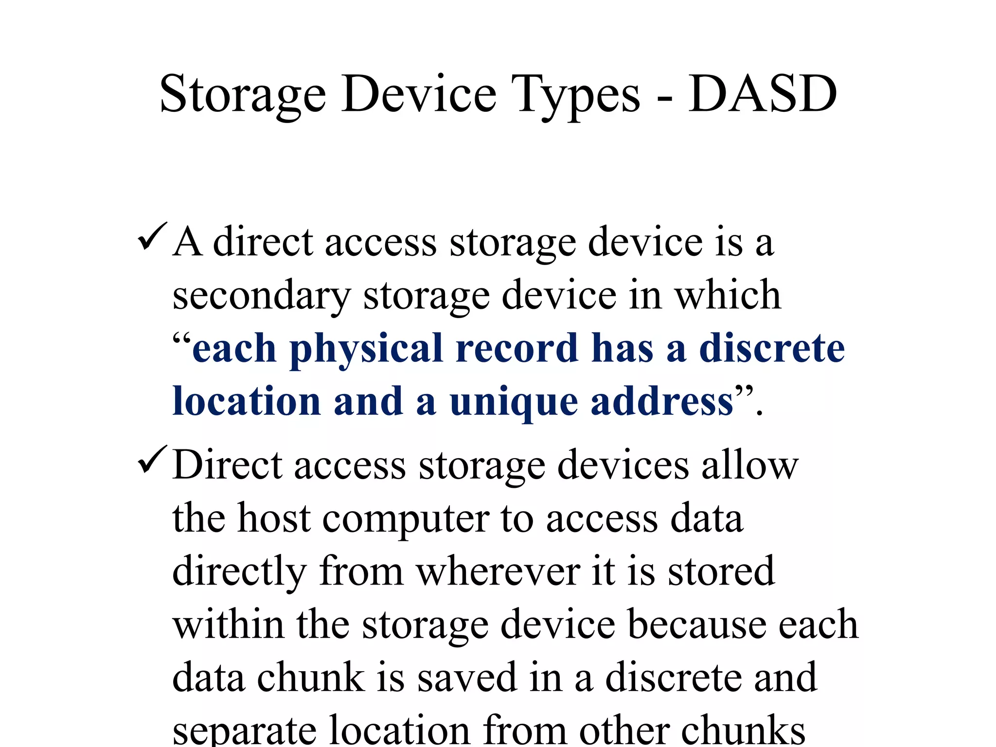
Storage Device Types- DASD
A direct access storage device is a
secondary storage device in which
“each physical record has a discrete
location and a unique address”.
Direct access storage devices allow
the host computer to access data
directly from wherever it is stored
within the storage device because each
data chunk is saved in a discrete and
separate location from other chunks
92.
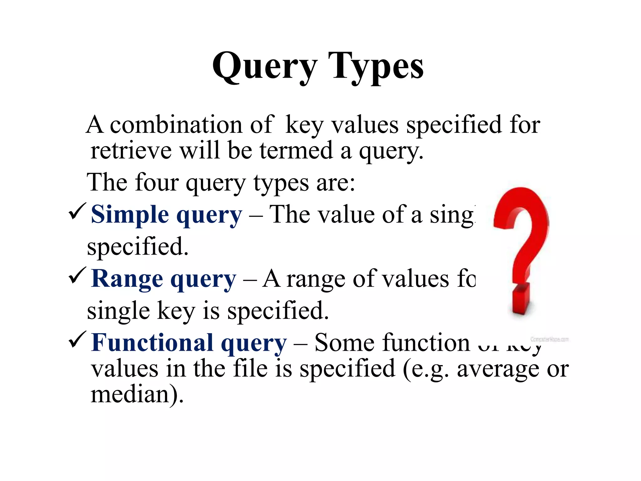
Query Types
A combinationof key values specified for
retrieve will be termed a query.
The four query types are:
Simple query – The value of a single key is
specified.
Range query – A range of values for a
single key is specified.
Functional query – Some function of key
values in the file is specified (e.g. average or
median).
93.
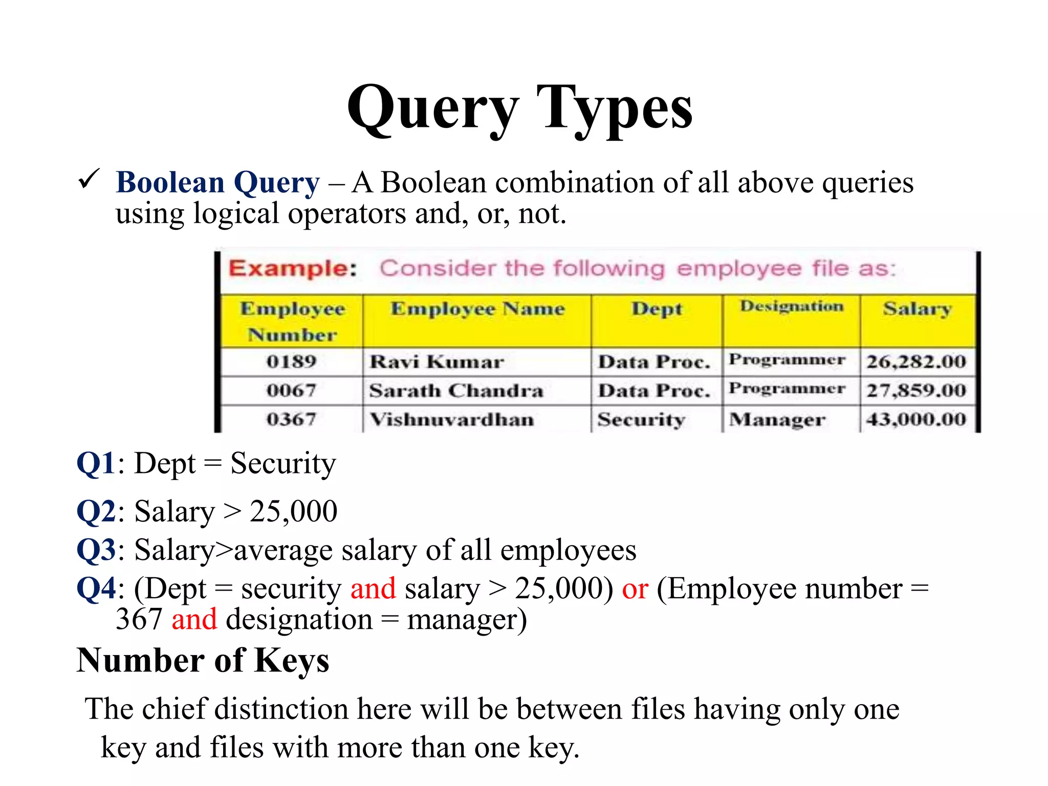
Boolean Query– A Boolean combination of all above queries
using logical operators and, or, not.
Q1: Dept = Security
Q2: Salary > 25,000
Q3: Salary>average salary of all employees
Q4: (Dept = security and salary > 25,000) or (Employee number =
367 and designation = manager)
Number of Keys
The chief distinction here will be between files having only one
key and files with more than one key.
Query Types
94.
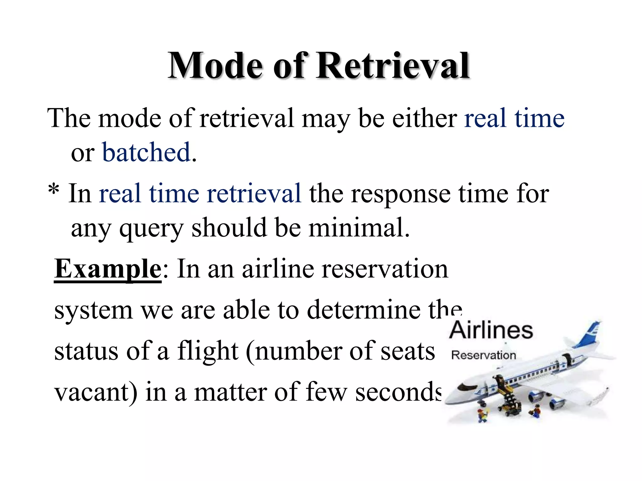
The mode ofretrieval may be either real time
or batched.
* In real time retrieval the response time for
any query should be minimal.
Example: In an airline reservation
system we are able to determine the
status of a flight (number of seats
vacant) in a matter of few seconds.
Mode of Retrieval
95.
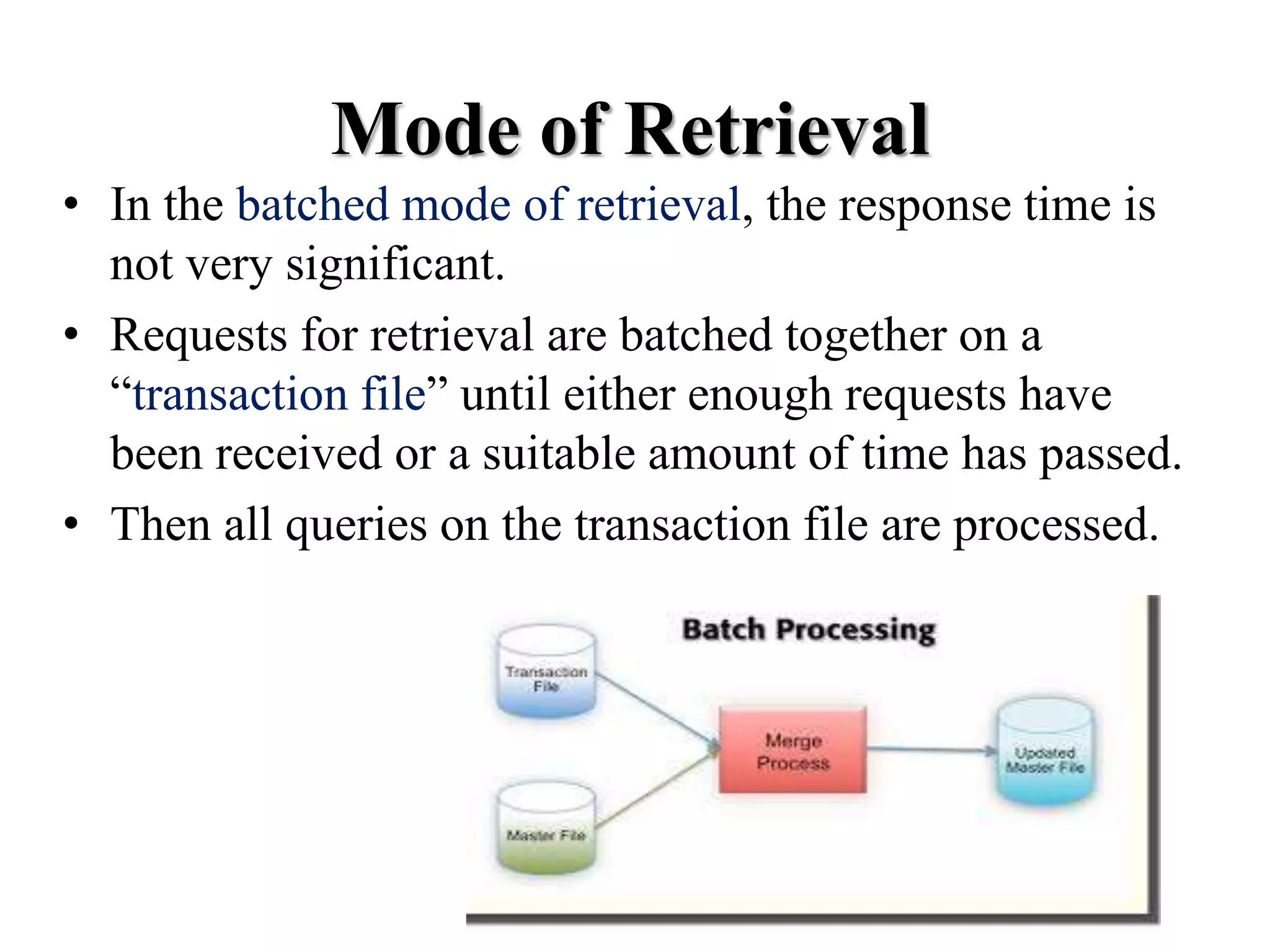
• In thebatched mode of retrieval, the response time is
not very significant.
• Requests for retrieval are batched together on a
“transaction file” until either enough requests have
been received or a suitable amount of time has passed.
• Then all queries on the transaction file are processed.
Mode of Retrieval
96.
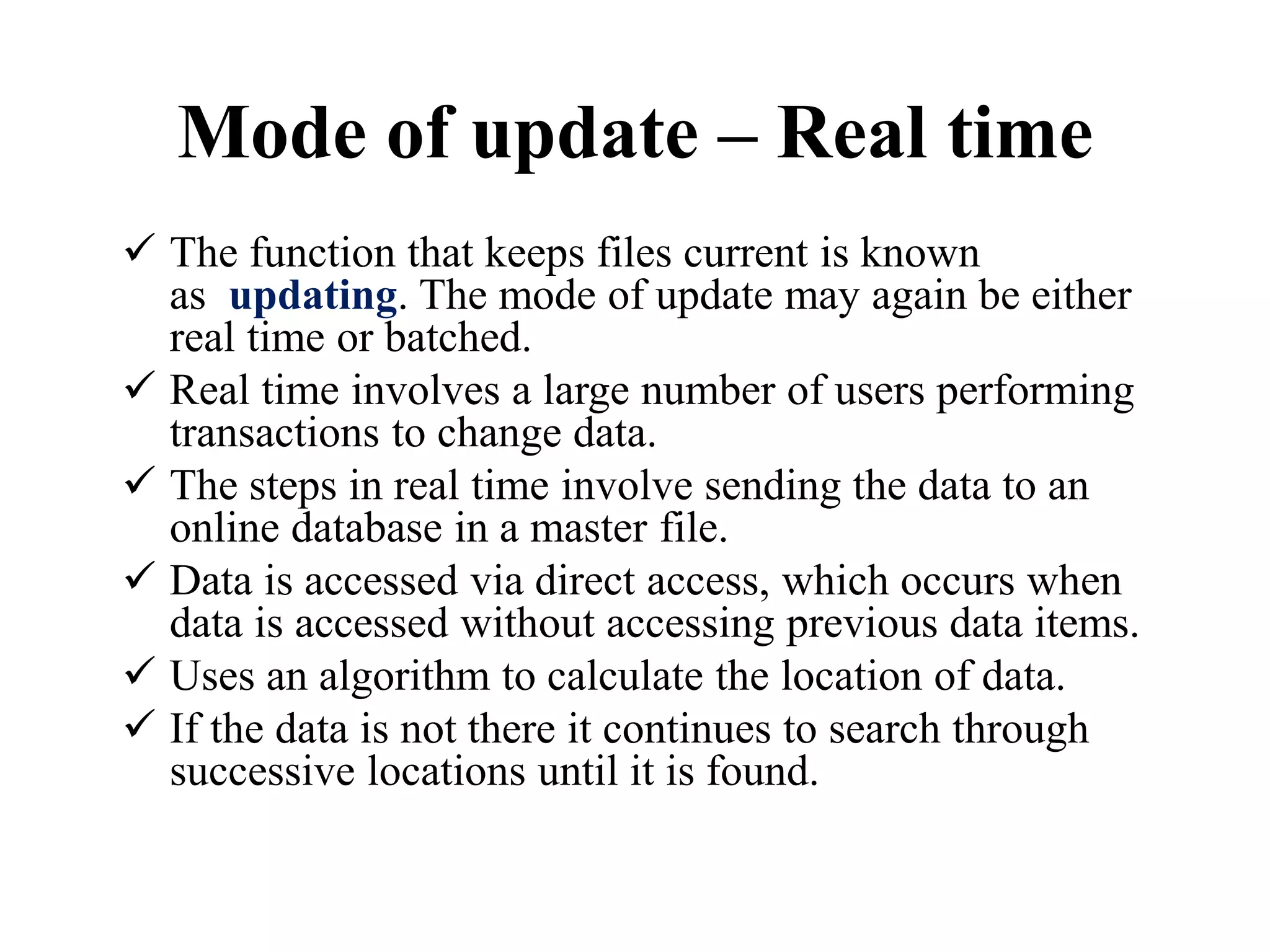
Mode of update– Real time
The function that keeps files current is known
as updating. The mode of update may again be either
real time or batched.
Real time involves a large number of users performing
transactions to change data.
The steps in real time involve sending the data to an
online database in a master file.
Data is accessed via direct access, which occurs when
data is accessed without accessing previous data items.
Uses an algorithm to calculate the location of data.
If the data is not there it continues to search through
successive locations until it is found.
97.
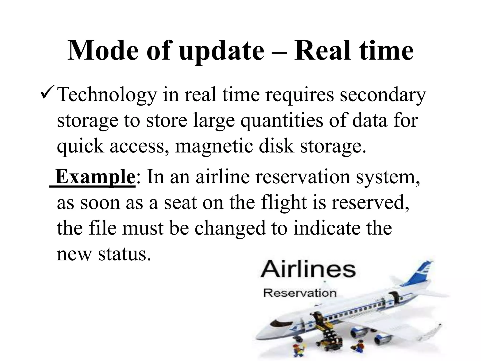
Technology in realtime requires secondary
storage to store large quantities of data for
quick access, magnetic disk storage.
Example: In an airline reservation system,
as soon as a seat on the flight is reserved,
the file must be changed to indicate the
new status.
Mode of update – Real time
98.
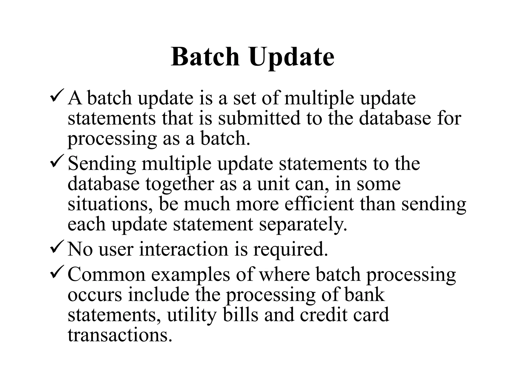
Batch Update
A batchupdate is a set of multiple update
statements that is submitted to the database for
processing as a batch.
Sending multiple update statements to the
database together as a unit can, in some
situations, be much more efficient than sending
each update statement separately.
No user interaction is required.
Common examples of where batch processing
occurs include the processing of bank
statements, utility bills and credit card
transactions.
99.
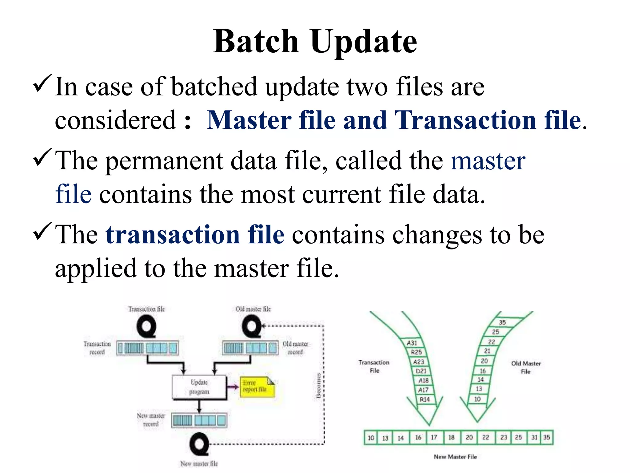
In case ofbatched update two files are
considered : Master file and Transaction file.
The permanent data file, called the master
file contains the most current file data.
The transaction file contains changes to be
applied to the master file.
Batch Update
100.
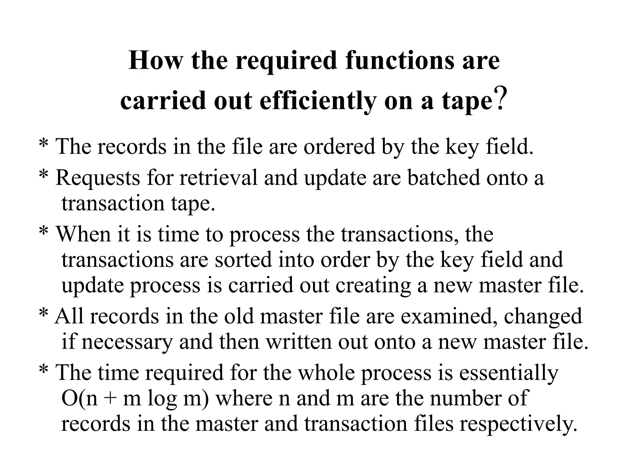
How the requiredfunctions are
carried out efficiently on a tape?
* The records in the file are ordered by the key field.
* Requests for retrieval and update are batched onto a
transaction tape.
* When it is time to process the transactions, the
transactions are sorted into order by the key field and
update process is carried out creating a new master file.
* All records in the old master file are examined, changed
if necessary and then written out onto a new master file.
* The time required for the whole process is essentially
O(n + m log m) where n and m are the number of
records in the master and transaction files respectively.
101.
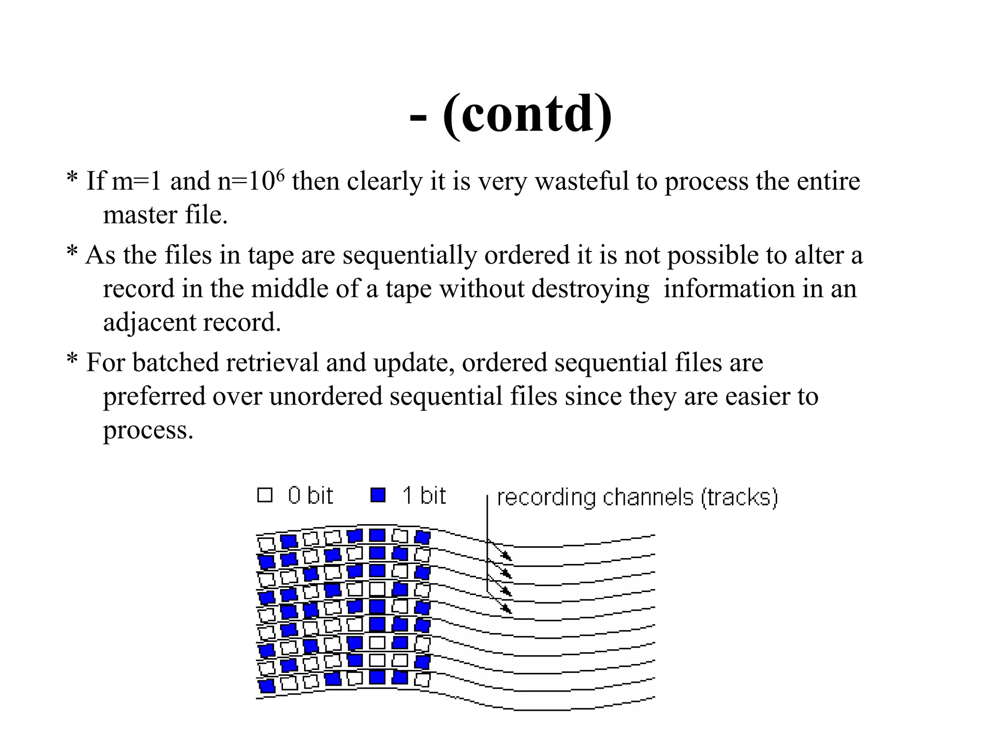
* If m=1and n=106 then clearly it is very wasteful to process the entire
master file.
* As the files in tape are sequentially ordered it is not possible to alter a
record in the middle of a tape without destroying information in an
adjacent record.
* For batched retrieval and update, ordered sequential files are
preferred over unordered sequential files since they are easier to
process.
- (contd)
102.
How the requiredfunctions are
carried out efficiently on a disk?
Batched retrieval and update can be carried out essentially
in the same way as for a sequentially ordered tape file by
setting up input and output buffers and reading in perhaps,
one track of the master and transaction files at a time.
The transaction file should be sorted on the primary key
before beginning the master file processing.
The sequential interpretation is particularly efficient for
batched update and retrieval as the tracks are to be accessed
in the order.
The read/write heads are moved one cylinder at a time and
this movement is necessitated only once for every s tracks
read (s = number of surfaces).
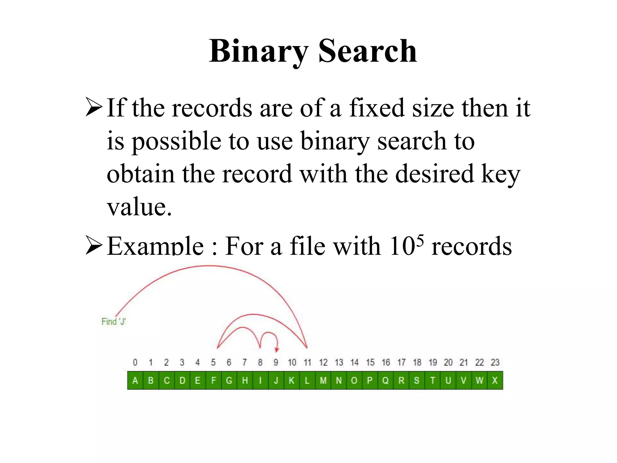
If the recordsare of a fixed size then it
is possible to use binary search to
obtain the record with the desired key
value.
Example : For a file with 105 records
of length 300 characters this would
mean a maximum of 17 accesses
Binary Search
105.
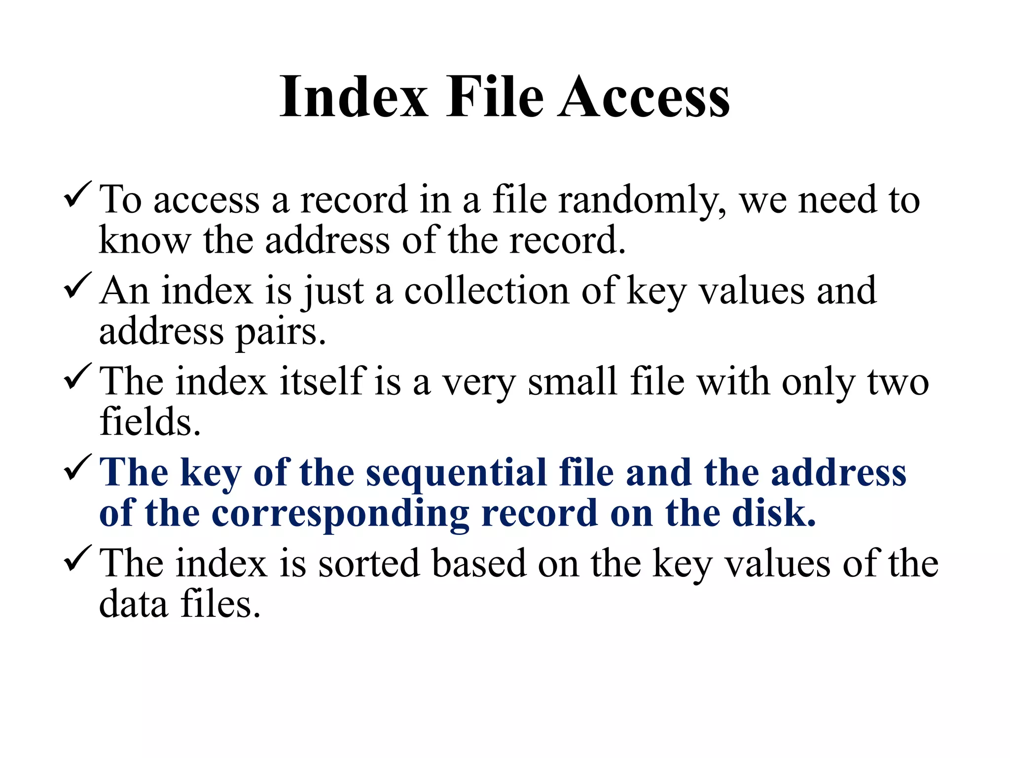
Index File Access
Toaccess a record in a file randomly, we need to
know the address of the record.
An index is just a collection of key values and
address pairs.
The index itself is a very small file with only two
fields.
The key of the sequential file and the address
of the corresponding record on the disk.
The index is sorted based on the key values of the
data files.
106.
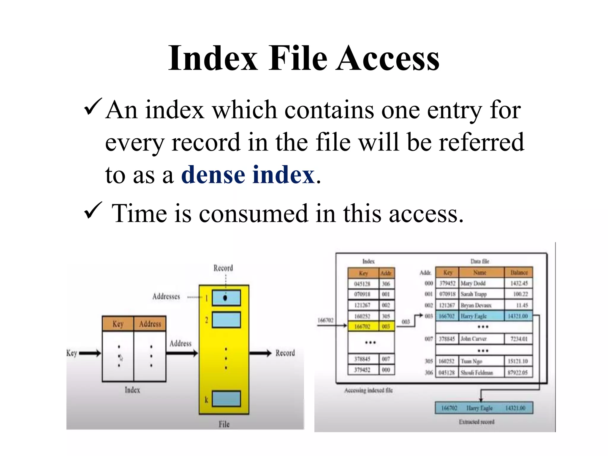
An index whichcontains one entry for
every record in the file will be referred
to as a dense index.
Time is consumed in this access.
Index File Access
107.
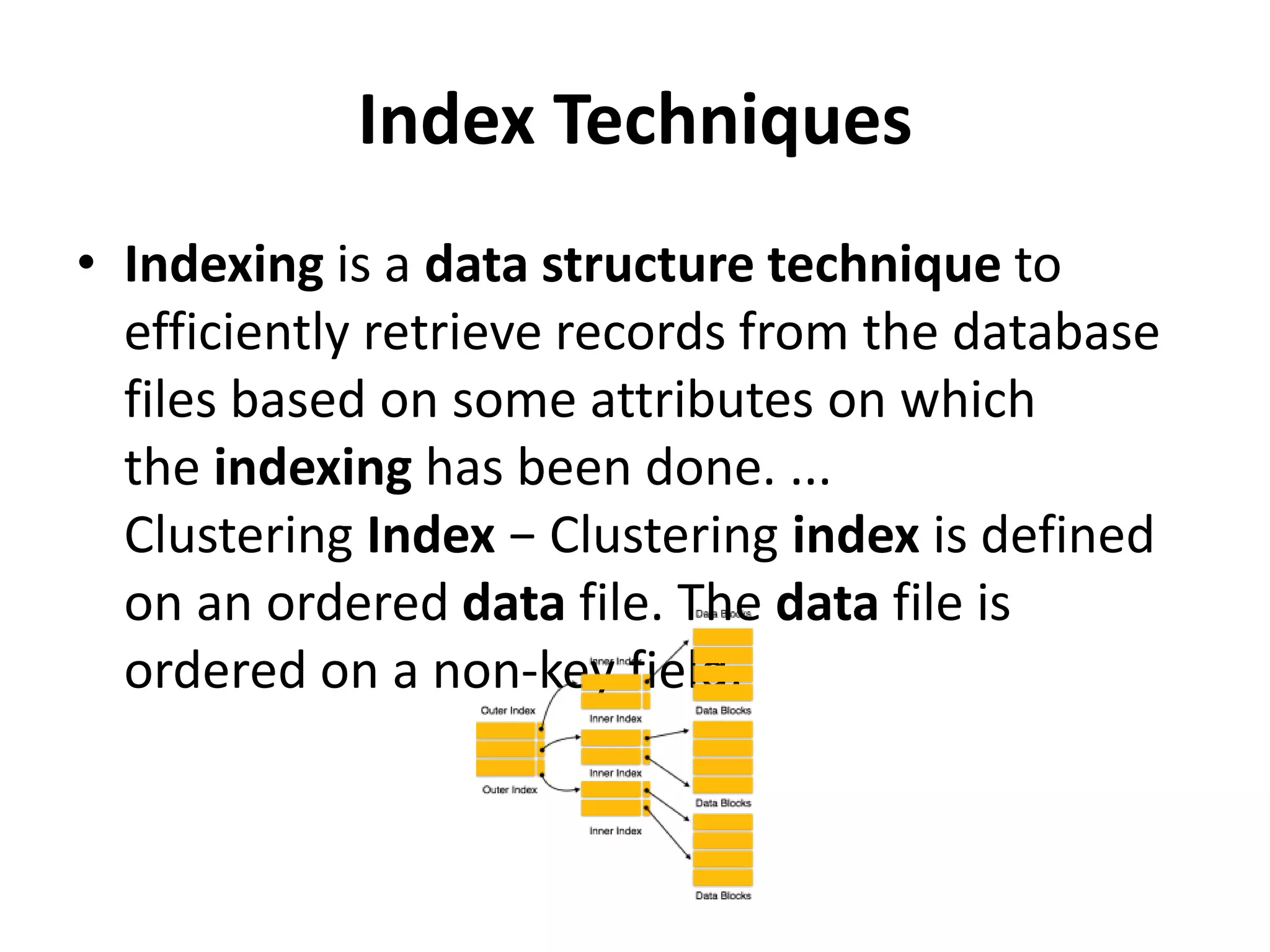
Index Techniques
• Indexingis a data structure technique to
efficiently retrieve records from the database
files based on some attributes on which
the indexing has been done. ...
Clustering Index − Clustering index is defined
on an ordered data file. The data file is
ordered on a non-key field.
108.
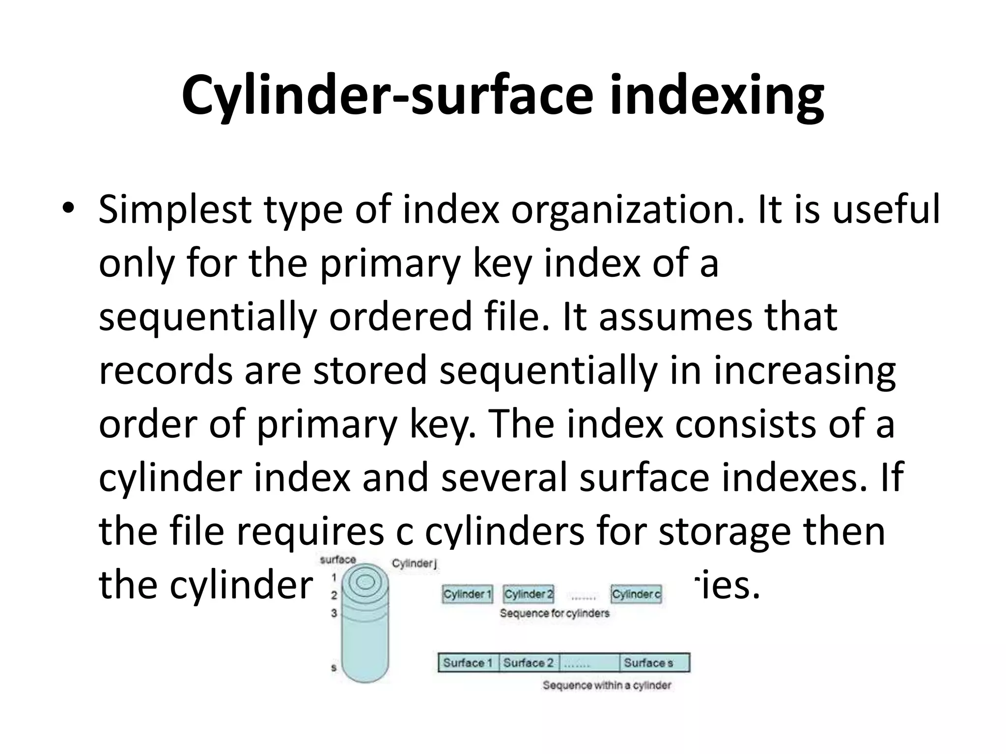
Cylinder-surface indexing
• Simplesttype of index organization. It is useful
only for the primary key index of a
sequentially ordered file. It assumes that
records are stored sequentially in increasing
order of primary key. The index consists of a
cylinder index and several surface indexes. If
the file requires c cylinders for storage then
the cylinder index contains c entries.
109.
Hashed indexes
• Hashfunctions and overflow handling techniques are
used for hashing. Since the index is to be maintained
on disk and disk access times are generally several
orders of magnitude larger than internal memory
access times, much consideration is given to hash table
design and the choice of an overflow handling
technique.
• Overflow handling techniques:
• rehashing
• open addressing (random[f(i)=random()], quadratic,
linear)
• chaining
110.
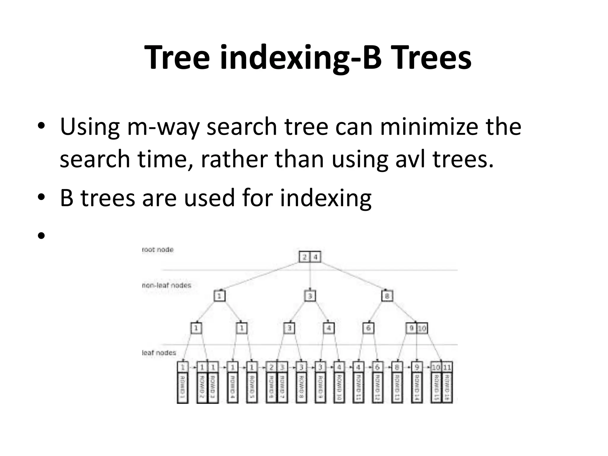
Tree indexing-B Trees
•Using m-way search tree can minimize the
search time, rather than using avl trees.
• B trees are used for indexing
•
111.
Trie indexing
• Anindex structure that is particularly useful
when key values are of varying size is trie.
• A trie is a tree of degree m>=2 in which the
branching at any level is determined not by
the entire key value but by only a portion of it.
• The trie contains two types of nodes. First
type called the branch node and second
information node.
File Organization
• Fileorganization refers to the way data is
stored in a file. File organization is very
important because it determines the methods
of access, efficiency, flexibility and storage
devices to use. There are four methods
of organizing files on a storage media.
114.
• What isFile?
• File is a collection of records related to each
other. The file size is limited by the size of
memory and storage medium.
• There are two important features of file:
1. File Activity
2. File Volatility
File Organization
115.
• File activityspecifies percent of actual records which proceed in a
single run.
File volatility addresses the properties of record changes. It helps to
increase the efficiency of disk design than tape.
• File Organization
File organization ensures that records are available for processing. It
is used to determine an efficient file organization for each base
relation.
For example, if we want to retrieve employee records in
alphabetical order of name. Sorting the file by employee name is a
good file organization. However, if we want to retrieve all
employees whose marks are in a certain range, a file is ordered by
employee name would not be a good file organization.
File Organization
116.
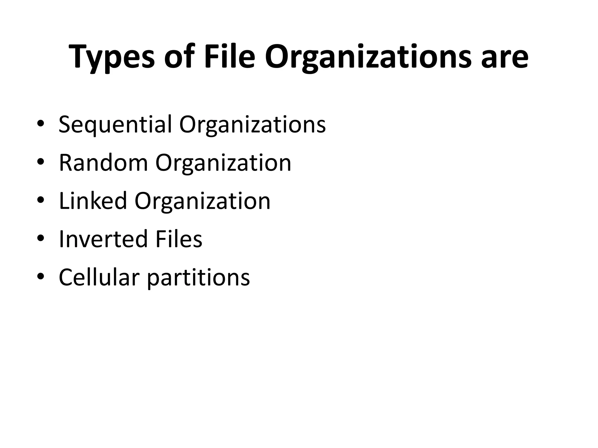
Types of FileOrganizations are
• Sequential Organizations
• Random Organization
• Linked Organization
• Inverted Files
• Cellular partitions
117.
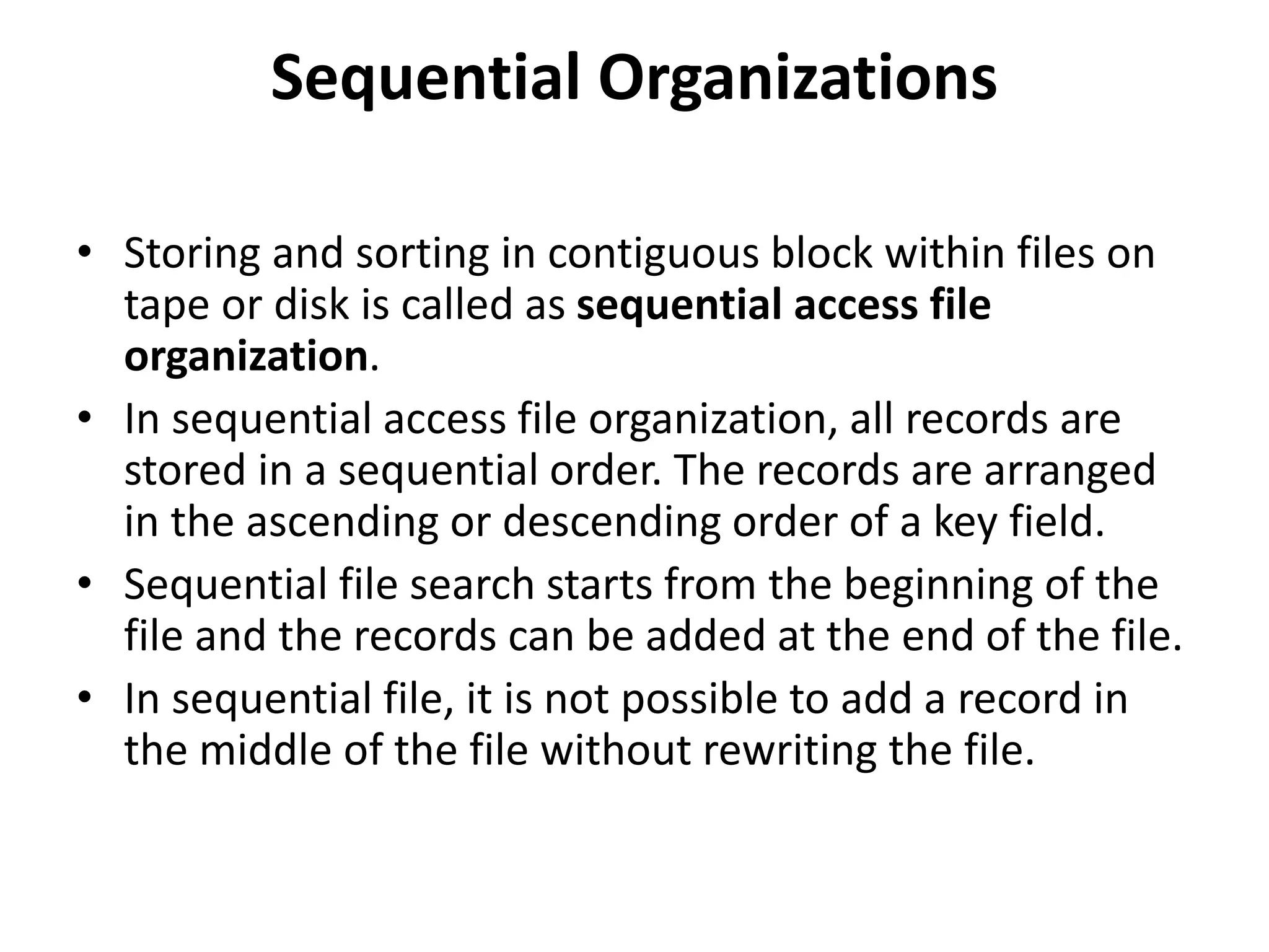
Sequential Organizations
• Storingand sorting in contiguous block within files on
tape or disk is called as sequential access file
organization.
• In sequential access file organization, all records are
stored in a sequential order. The records are arranged
in the ascending or descending order of a key field.
• Sequential file search starts from the beginning of the
file and the records can be added at the end of the file.
• In sequential file, it is not possible to add a record in
the middle of the file without rewriting the file.
118.
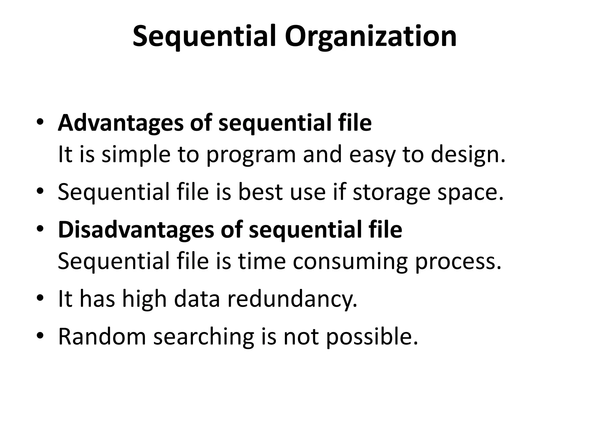
• Advantages ofsequential file
It is simple to program and easy to design.
• Sequential file is best use if storage space.
• Disadvantages of sequential file
Sequential file is time consuming process.
• It has high data redundancy.
• Random searching is not possible.
Sequential Organization
119.
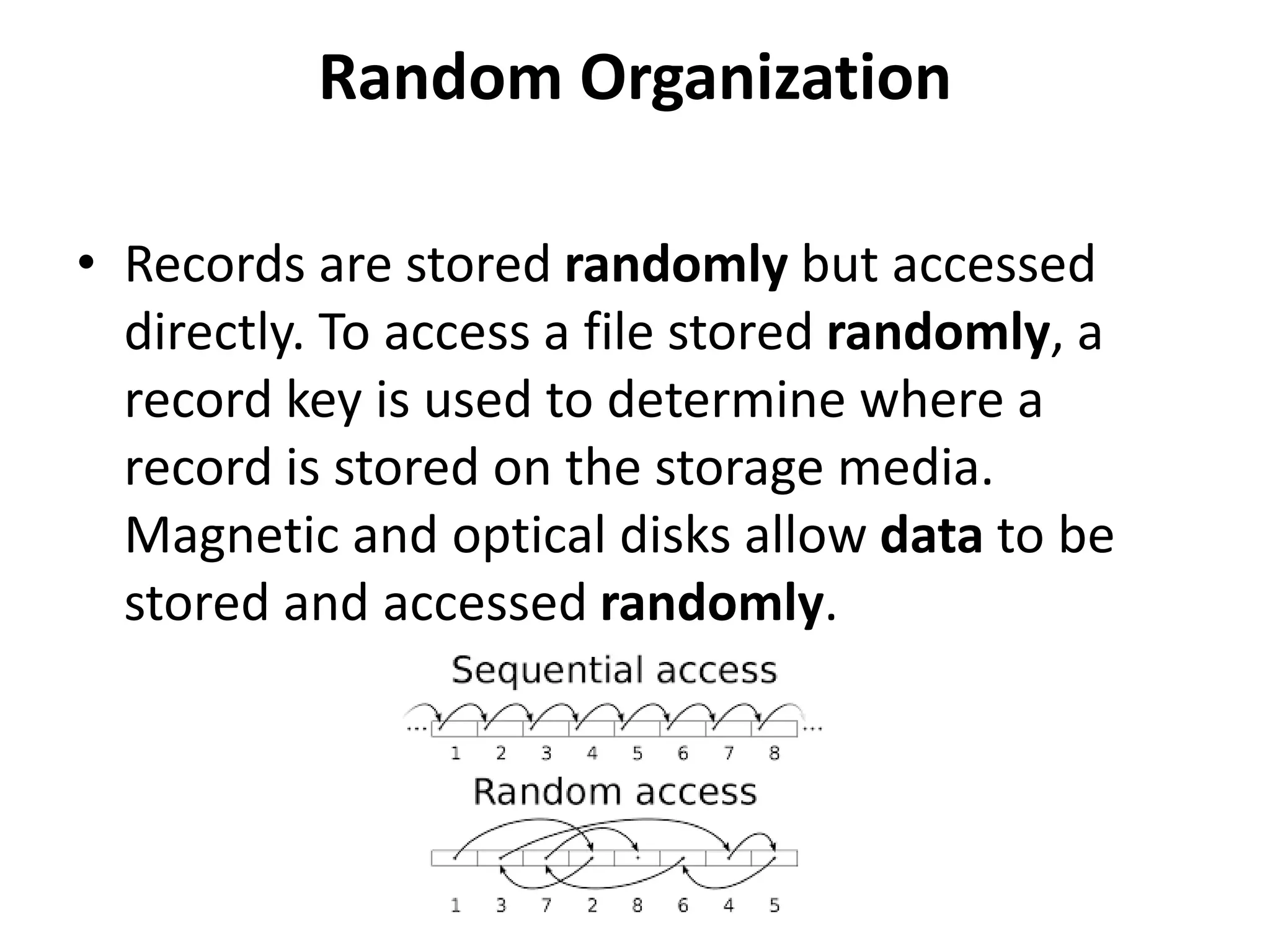
Random Organization
• Recordsare stored randomly but accessed
directly. To access a file stored randomly, a
record key is used to determine where a
record is stored on the storage media.
Magnetic and optical disks allow data to be
stored and accessed randomly.
120.
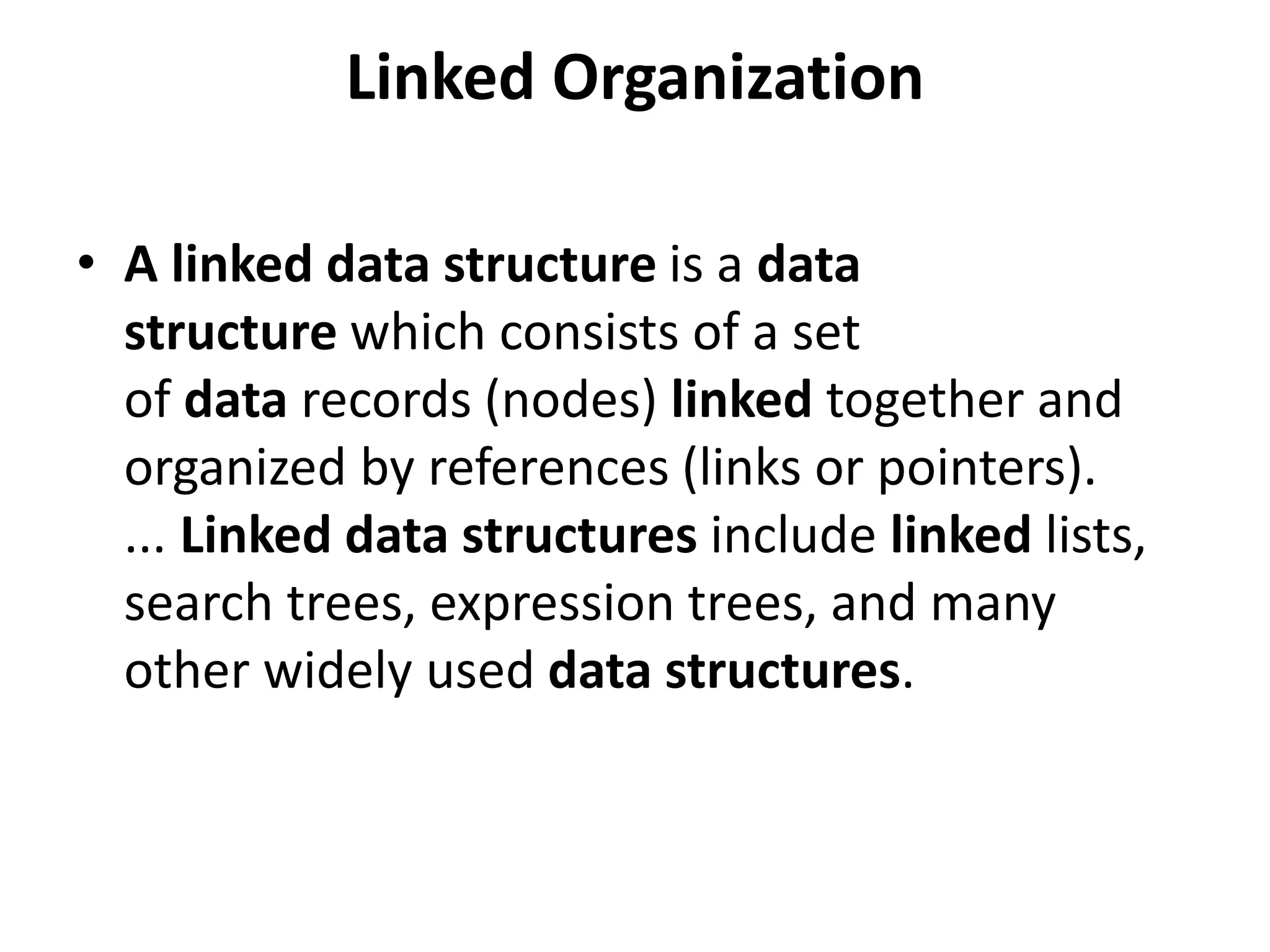
Linked Organization
• Alinked data structure is a data
structure which consists of a set
of data records (nodes) linked together and
organized by references (links or pointers).
... Linked data structures include linked lists,
search trees, expression trees, and many
other widely used data structures.
121.
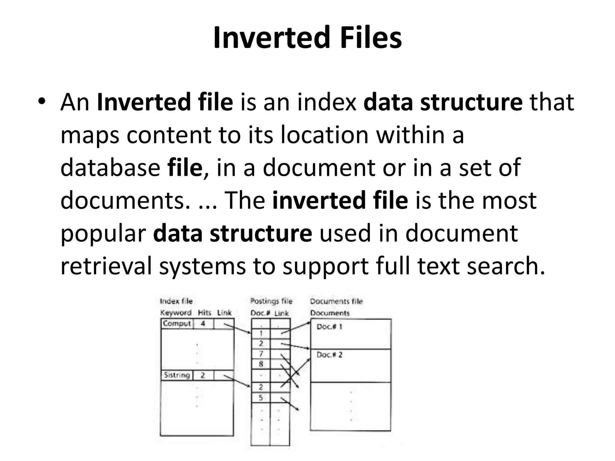
Inverted Files
• AnInverted file is an index data structure that
maps content to its location within a
database file, in a document or in a set of
documents. ... The inverted file is the most
popular data structure used in document
retrieval systems to support full text search.
122.
Cellular partitions
• Toreduce the file search times, the storage
media may be divided into cells. A cell may be
an entire disk pack or it may simply be a
cylinder. Lists are localized to lie within a cell.
![Insertion Sort
• Example 7.1: Assume n = 5 and the input sequence is (5,4,3,2,1) [note the
records have only one field which also happens to be the key]. Then, after
each insertion we have the following:
Note that this is an example of the worst case behavior.
• Example 7.2: n = 5 and the input sequence is (2, 3, 4, 5, 1). After each
execution of INSERT we have:](https://image.slidesharecdn.com/unit5-internalsortingfiles-201110061740/75/Unit-5-internal-sorting-amp-files-10-2048.jpg)
![Example
We are given array of n integers to sort:
40 20 10 80 60 50 7 30 100
[0] [1] [2] [3] [4] [5] [6] [7] [8]](https://image.slidesharecdn.com/unit5-internalsortingfiles-201110061740/75/Unit-5-internal-sorting-amp-files-17-2048.jpg)
![Pick Pivot Element
There are a number of ways to pick the pivot element. In
this example, we will use the first element in the array:
40 20 10 80 60 50 7 30 100
[0] [1] [2] [3] [4] [5] [6] [7] [8]](https://image.slidesharecdn.com/unit5-internalsortingfiles-201110061740/75/Unit-5-internal-sorting-amp-files-18-2048.jpg)
![40 20 10 80 60 50 7 30 100pivot_index = 0
i j
[0] [1] [2] [3] [4] [5] [6] [7] [8]](https://image.slidesharecdn.com/unit5-internalsortingfiles-201110061740/75/Unit-5-internal-sorting-amp-files-19-2048.jpg)
![40 20 10 80 60 50 7 30 100pivot_index = 0
[0] [1] [2] [3] [4] [5] [6] [7] [8]
i j
1. While data[i] <= data[pivot]
++ i](https://image.slidesharecdn.com/unit5-internalsortingfiles-201110061740/75/Unit-5-internal-sorting-amp-files-20-2048.jpg)
![40 20 10 80 60 50 7 30 100pivot_index = 0
i j
1. While data[i] <= data[pivot]
++ i
[0] [1] [2] [3] [4] [5] [6] [7] [8]](https://image.slidesharecdn.com/unit5-internalsortingfiles-201110061740/75/Unit-5-internal-sorting-amp-files-21-2048.jpg)
![40 20 10 80 60 50 7 30 100pivot_index = 0
i j
1. While data[i] <= data[pivot]
++ i
[0] [1] [2] [3] [4] [5] [6] [7] [8]](https://image.slidesharecdn.com/unit5-internalsortingfiles-201110061740/75/Unit-5-internal-sorting-amp-files-22-2048.jpg)
![40 20 10 80 60 50 7 30 100pivot_index = 0
i j
1. While data[i] <= data[pivot]
++ i
2. While data[j] > data[pivot]
--j
[0] [1] [2] [3] [4] [5] [6] [7] [8]](https://image.slidesharecdn.com/unit5-internalsortingfiles-201110061740/75/Unit-5-internal-sorting-amp-files-23-2048.jpg)
![40 20 10 80 60 50 7 30 100pivot_index = 0
i j
1. While data[i] <= data[pivot]
++ i
2. While data[j] > data[pivot]
--j
[0] [1] [2] [3] [4] [5] [6] [7] [8]](https://image.slidesharecdn.com/unit5-internalsortingfiles-201110061740/75/Unit-5-internal-sorting-amp-files-24-2048.jpg)
![40 20 10 80 60 50 7 30 100pivot_index = 0
i j
1. While data[i] <= data[pivot]
++ i
2. While data[j] > data[pivot]
--j
3. If i > j
swap data[i] and data[j]
[0] [1] [2] [3] [4] [5] [6] [7] [8]](https://image.slidesharecdn.com/unit5-internalsortingfiles-201110061740/75/Unit-5-internal-sorting-amp-files-25-2048.jpg)
![40 20 10 30 60 50 7 80 100pivot_index = 0
i j
1. While data[i] <= data[pivot]
++ i
2. While data[j] > data[pivot]
--j
3. If i > j
swap data[i] and data[j]
[0] [1] [2] [3] [4] [5] [6] [7] [8]](https://image.slidesharecdn.com/unit5-internalsortingfiles-201110061740/75/Unit-5-internal-sorting-amp-files-26-2048.jpg)
![40 20 10 30 60 50 7 80 100pivot_index = 0
i j
1. While data[i] <= data[pivot]
++ i
2. While data[j] > data[pivot]
--j
3. If i > j
swap data[i] and data[j]
4. While j > i, go to 1.
[0] [1] [2] [3] [4] [5] [6] [7] [8]](https://image.slidesharecdn.com/unit5-internalsortingfiles-201110061740/75/Unit-5-internal-sorting-amp-files-27-2048.jpg)
![40 20 10 30 60 50 7 80 100pivot_index = 0
i j
1. While data[i] <= data[pivot]
++ i
2. While data[j] > data[pivot]
--j
3. If i > j
swap data[i] and data[j]
4. While j> i, go to 1.
[0] [1] [2] [3] [4] [5] [6] [7] [8]](https://image.slidesharecdn.com/unit5-internalsortingfiles-201110061740/75/Unit-5-internal-sorting-amp-files-28-2048.jpg)
![40 20 10 30 60 50 7 80 100pivot_index = 0
i j
1. While data[i] <= data[pivot]
++ i
2. While data[j] > data[pivot]
--j
3. If i > j
swap data[i] and [j]
4. While j> i, go to 1.
[0] [1] [2] [3] [4] [5] [6] [7] [8]](https://image.slidesharecdn.com/unit5-internalsortingfiles-201110061740/75/Unit-5-internal-sorting-amp-files-29-2048.jpg)
![40 20 10 30 60 50 7 80 100pivot_index = 0
i j
1. While data[i] <= data[pivot]
++ i
2. While data[j] > data[pivot]
--j
3. If i > j
swap data[i] and data[j]
4. While j> i, go to 1.
[0] [1] [2] [3] [4] [5] [6] [7] [8]](https://image.slidesharecdn.com/unit5-internalsortingfiles-201110061740/75/Unit-5-internal-sorting-amp-files-30-2048.jpg)
![40 20 10 30 60 50 7 80 100pivot_index = 0
i j
1. While data[i] <= data[pivot]
++ i
2. While data[j] > data[pivot]
--j
3. If i > j
swap data[i] and data[j]
4. While j > i, go to 1.
[0] [1] [2] [3] [4] [5] [6] [7] [8]](https://image.slidesharecdn.com/unit5-internalsortingfiles-201110061740/75/Unit-5-internal-sorting-amp-files-31-2048.jpg)
![40 20 10 30 60 50 7 80 100pivot_index = 0
i j
1. While data[i] <= data[pivot]
++ i
2. While data[j] > data[pivot]
--j
3. If i > j
swap data[i] and data[j]
4. While j > i, go to 1.
[0] [1] [2] [3] [4] [5] [6] [7] [8]](https://image.slidesharecdn.com/unit5-internalsortingfiles-201110061740/75/Unit-5-internal-sorting-amp-files-32-2048.jpg)
![1. While data[i] <= data[pivot]
++ i
2. While data[j] > data[pivot]
--j
3. If i > j
swap data[i] and data[j]
4. While j > i, go to 1.
40 20 10 30 7 50 60 80 100pivot_index = 0
i j
[0] [1] [2] [3] [4] [5] [6] [7] [8]](https://image.slidesharecdn.com/unit5-internalsortingfiles-201110061740/75/Unit-5-internal-sorting-amp-files-33-2048.jpg)
![1. While data[i] <= data[pivot]
++i
2. While data[j] > data[pivot]
--j
3. If i > j
swap data[i] and data[j]
4. While j > i, go to 1.
40 20 10 30 7 50 60 80 100pivot_index = 0
i j
[0] [1] [2] [3] [4] [5] [6] [7] [8]](https://image.slidesharecdn.com/unit5-internalsortingfiles-201110061740/75/Unit-5-internal-sorting-amp-files-34-2048.jpg)
![1. While data[i] <= data[pivot]
++i
2. While data[j] > data[pivot]
--j
3. If i > j
swap data[i] and data[j]
4. While j > i, go to 1.
40 20 10 30 7 50 60 80 100pivot_index = 0
i j
[0] [1] [2] [3] [4] [5] [6] [7] [8]](https://image.slidesharecdn.com/unit5-internalsortingfiles-201110061740/75/Unit-5-internal-sorting-amp-files-35-2048.jpg)
![1. While data[i] <= data[pivot]
++i
2. While data[j] > data[pivot]
--j
3. If i > j
swap data[i] and data[j]
4. While j > i, go to 1.
40 20 10 30 7 50 60 80 100pivot_index = 0
i j
[0] [1] [2] [3] [4] [5] [6] [7] [8]](https://image.slidesharecdn.com/unit5-internalsortingfiles-201110061740/75/Unit-5-internal-sorting-amp-files-36-2048.jpg)
![1. While data[i] <= data[pivot]
++i
2. While data[j] > data[pivot]
--j
3. If i > j
swap data[i] and data[j]
4. While j > i, go to 1.
40 20 10 30 7 50 60 80 100pivot_index = 0
i j
[0] [1] [2] [3] [4] [5] [6] [7] [8]](https://image.slidesharecdn.com/unit5-internalsortingfiles-201110061740/75/Unit-5-internal-sorting-amp-files-37-2048.jpg)
![1. While data[i] <= data[pivot]
++i
2. While data[j] > data[pivot]
--j
3. If i > j
swap data[i] and data[j]
4. While j > i, go to 1.
40 20 10 30 7 50 60 80 100pivot_index = 0
i j
[0] [1] [2] [3] [4] [5] [6] [7] [8]](https://image.slidesharecdn.com/unit5-internalsortingfiles-201110061740/75/Unit-5-internal-sorting-amp-files-38-2048.jpg)
![1. While data[i] <= data[pivot]
++i
2. While data[j] > data[pivot]
--j
3. If i > j
swap data[i] and data[j]
4. While j > i, go to 1.
40 20 10 30 7 50 60 80 100pivot_index = 0
i j
[0] [1] [2] [3] [4] [5] [6] [7] [8]](https://image.slidesharecdn.com/unit5-internalsortingfiles-201110061740/75/Unit-5-internal-sorting-amp-files-39-2048.jpg)
![1. While data[i] <= data[pivot]
++i
2. While data[j] > data[pivot]
--j
3. If i > j
swap data[i] and data[j]
4. While j > i, go to 1.
40 20 10 30 7 50 60 80 100pivot_index = 0
i j
[0] [1] [2] [3] [4] [5] [6] [7] [8]](https://image.slidesharecdn.com/unit5-internalsortingfiles-201110061740/75/Unit-5-internal-sorting-amp-files-40-2048.jpg)
![1. While data[i] <= data[pivot]
++i
2. While data[j] > data[pivot]
--j
3. If i > j
swap data[i] and data[j]
4. While j > i, go to 1.
40 20 10 30 7 50 60 80 100pivot_index = 0
i j
[0] [1] [2] [3] [4] [5] [6] [7] [8]](https://image.slidesharecdn.com/unit5-internalsortingfiles-201110061740/75/Unit-5-internal-sorting-amp-files-41-2048.jpg)
![1. While data[i] <= data[pivot]
++i
2. While data[j] > data[pivot]
--j
3. If i > j
swap data[i] and data[j]
4. While j > i, go to 1.
5. Swap data[j] and data[pivot_index]
40 20 10 30 7 50 60 80 100pivot_index = 0
i j
[0] [1] [2] [3] [4] [5] [6] [7] [8]](https://image.slidesharecdn.com/unit5-internalsortingfiles-201110061740/75/Unit-5-internal-sorting-amp-files-42-2048.jpg)
![1. While data[i] <= data[pivot]
++i
2. While data[j] > data[pivot]
--j
3. If i > j
swap data[i] and data[j]
4. While j > i, go to 1.
5. Swap data[j] and data[pivot_index]
7 20 10 30 40 50 60 80 100pivot_index = 4
i j
[0] [1] [2] [3] [4] [5] [6] [7] [8]](https://image.slidesharecdn.com/unit5-internalsortingfiles-201110061740/75/Unit-5-internal-sorting-amp-files-43-2048.jpg)
![Partition Result
7 20 10 30 40 50 60 80 100
<= data[pivot] > data[pivot]
[0] [1] [2] [3] [4] [5] [6] [7] [8]](https://image.slidesharecdn.com/unit5-internalsortingfiles-201110061740/75/Unit-5-internal-sorting-amp-files-44-2048.jpg)
![Quick Sort Algorithm
In Quick sort algorithm, partitioning of the list is performed using
following steps...
Step 1 - Consider the first element of the list as pivot (i.e., Element at
first position in the list).
Step 2 - Define two variables i and j. Set i and j to first and last elements
of the list respectively.
Step 3 - Increment i until list[i] > pivot then stop.
Step 4 - Decrement j until list[j] < pivot then stop.
Step 5 - If i > j then exchange list[i] and list[j].
Step 6 - Repeat steps 3,4 & 5 until I < j.
Step 7 - Exchange the pivot element with list[j] element.](https://image.slidesharecdn.com/unit5-internalsortingfiles-201110061740/75/Unit-5-internal-sorting-amp-files-45-2048.jpg)
![Quick Sort
40 20 10 80 60 50 7 30 100
[0] [1] [2] [3] [4] [5] [6] [7] [8]
m n
K = Pivot
Ki
Kj
i
j
m nj-1
j
j+1](https://image.slidesharecdn.com/unit5-internalsortingfiles-201110061740/75/Unit-5-internal-sorting-amp-files-47-2048.jpg)
![Merge-Sort
• An execution of merge-sort is depicted by a binary
tree
– each node represents a recursive call of merge-sort and
stores
– the root is the initial call
– the leaves are calls on subsequences of size 0 or 1
• Given two sorted lists
(list[i], …, list[m])
(list[m+1], …, list[n])
generate a single sorted list
(sorted[i], …, sorted[n])
• O(n) space vs. O(1) space
Merge Sort 50](https://image.slidesharecdn.com/unit5-internalsortingfiles-201110061740/75/Unit-5-internal-sorting-amp-files-50-2048.jpg)
![Example -2
• Partition into lists of size n/2
[10, 4, 6, 3]
[10, 4, 6, 3, 8, 2, 5, 7]
[8, 2, 5, 7]
[10, 4] [6, 3] [8, 2] [5, 7]
[10] [4] [6] [3] [8] [2] [5] [7]](https://image.slidesharecdn.com/unit5-internalsortingfiles-201110061740/75/Unit-5-internal-sorting-amp-files-63-2048.jpg)
![Example- 2 Cont’d
• Merge
[3, 4, 6, 10]
[2, 3, 4, 5, 6, 7, 8, 10 ]
[2, 5, 7, 8]
[4, 10] [3, 6] [2, 8] [5, 7]
[10] [4] [6] [3] [8] [2] [5] [7]](https://image.slidesharecdn.com/unit5-internalsortingfiles-201110061740/75/Unit-5-internal-sorting-amp-files-64-2048.jpg)
![Merge Sort
[3, 4, 6, 10]
[2, 3, 4, 5, 6, 7, 8, 10 ]
[2, 5, 7, 8]
[10, 4, 6, 3, 8, 2, 5, 7]Input Array
Output Array (Sorted)
X X
K
Xi Xj
Zk](https://image.slidesharecdn.com/unit5-internalsortingfiles-201110061740/75/Unit-5-internal-sorting-amp-files-65-2048.jpg)
![Heap Sort
50 10 23 1 7 -4
Initial
Array
[0] [1] [2] [3] [4] [5]](https://image.slidesharecdn.com/unit5-internalsortingfiles-201110061740/75/Unit-5-internal-sorting-amp-files-69-2048.jpg)
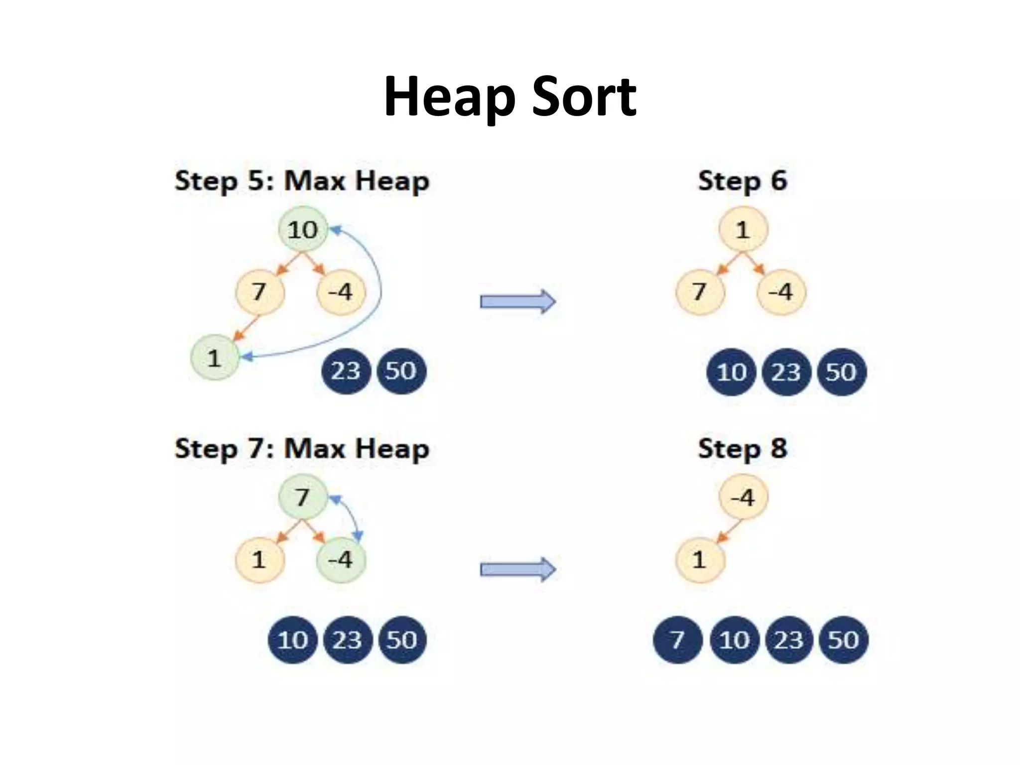
![Heap Sort
-4 1 7 10 23 50
Sorted
Array
[0] [1] [2] [3] [4] [5]](https://image.slidesharecdn.com/unit5-internalsortingfiles-201110061740/75/Unit-5-internal-sorting-amp-files-71-2048.jpg)
![Procedure -Heap
15 5 20 1 17 10 30
[1] [2] [3] [4] [5] [6] [7]](https://image.slidesharecdn.com/unit5-internalsortingfiles-201110061740/75/Unit-5-internal-sorting-amp-files-72-2048.jpg)
![Shell Sort Algorithm
1.shellsort(int arr[], int num)
2.{
3.int i, j, k;
4.for (i = num / 2; i > 0; i = i / 2)
5.{
6.for (j = i; j < num; j++)
7.{
8.for(k = j - i; k >= 0; k = k - i)
9.{
10.if (arr[k+i] >= arr[k])
11.break;
12.else
13.{
14.Swap arr[k] =
arr[k+i];}
15.}
16.}
17.}
18.}](https://image.slidesharecdn.com/unit5-internalsortingfiles-201110061740/75/Unit-5-internal-sorting-amp-files-83-2048.jpg)


![Hashed indexes
• Hash functions and overflow handling techniques are
used for hashing. Since the index is to be maintained
on disk and disk access times are generally several
orders of magnitude larger than internal memory
access times, much consideration is given to hash table
design and the choice of an overflow handling
technique.
• Overflow handling techniques:
• rehashing
• open addressing (random[f(i)=random()], quadratic,
linear)
• chaining](https://image.slidesharecdn.com/unit5-internalsortingfiles-201110061740/75/Unit-5-internal-sorting-amp-files-109-2048.jpg)


![Data Structures - Lecture 8 [Sorting Algorithms]](https://cdn.slidesharecdn.com/ss_thumbnails/lecture-8sortingalgorithms-150205105023-conversion-gate02-thumbnail.jpg?width=640&height=640&fit=bounds)


![Data Structures - Lecture 1 [introduction]](https://cdn.slidesharecdn.com/ss_thumbnails/lecture-1introduction-141217054305-conversion-gate02-thumbnail.jpg?width=640&height=640&fit=bounds)