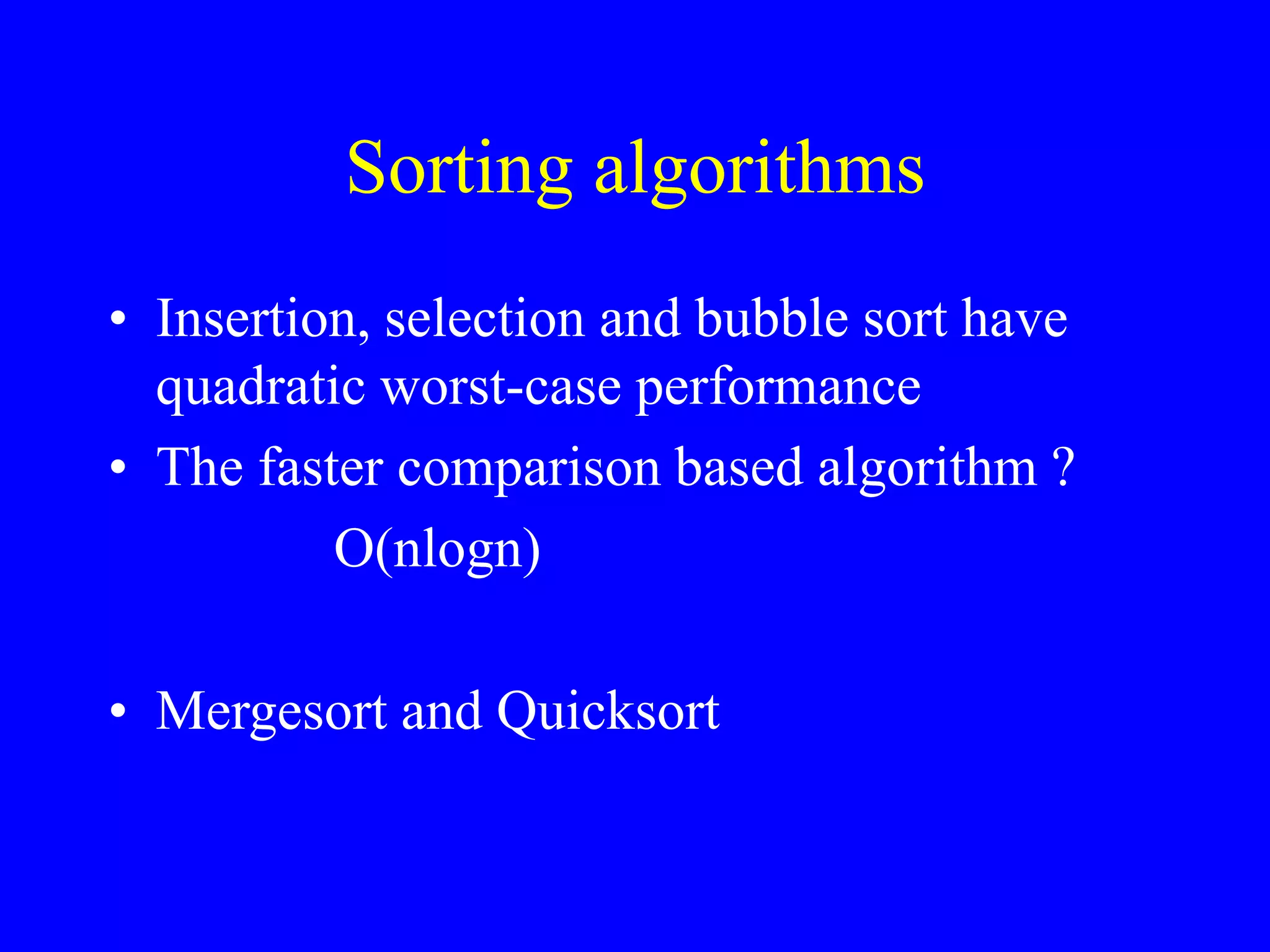
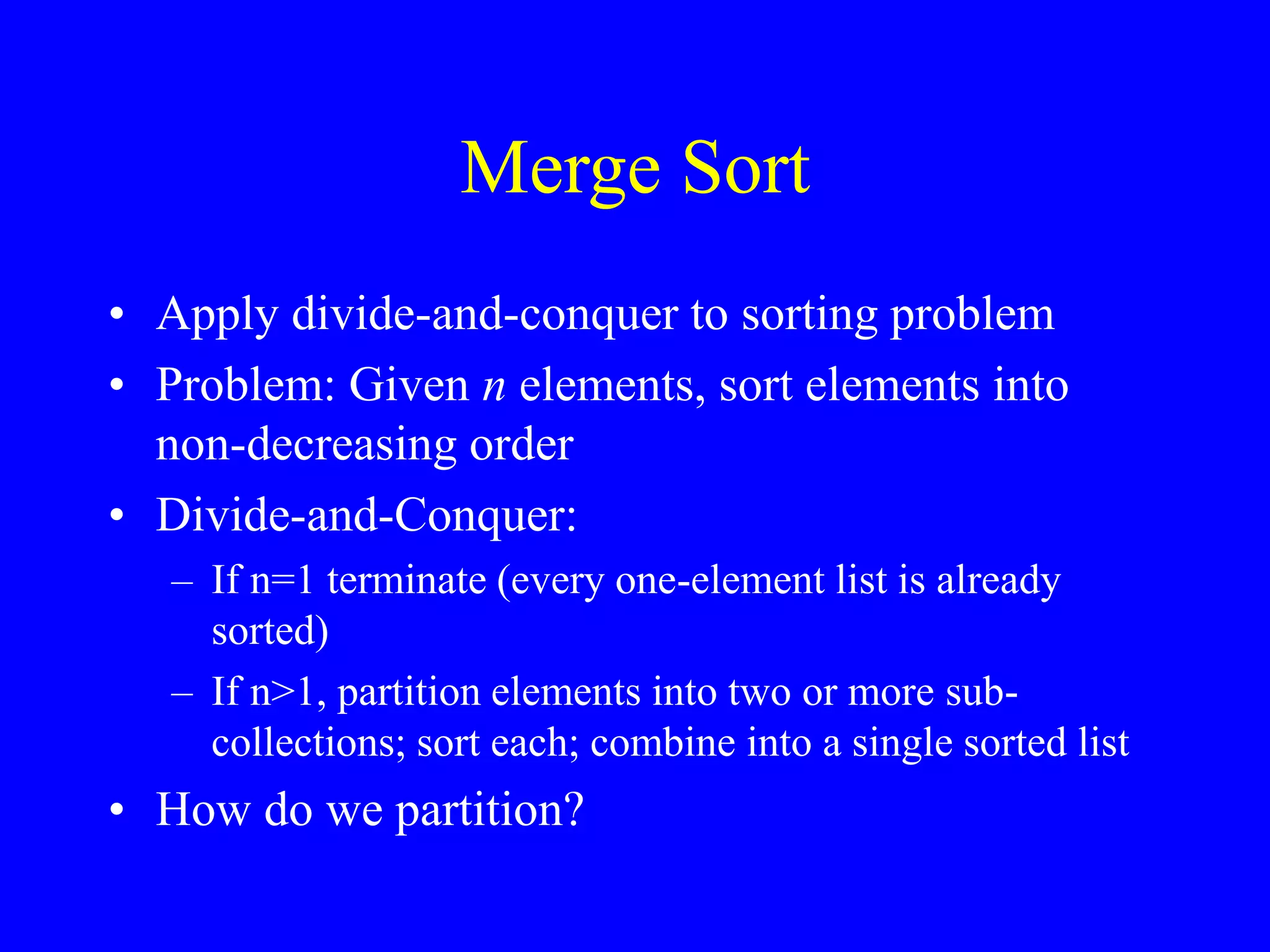
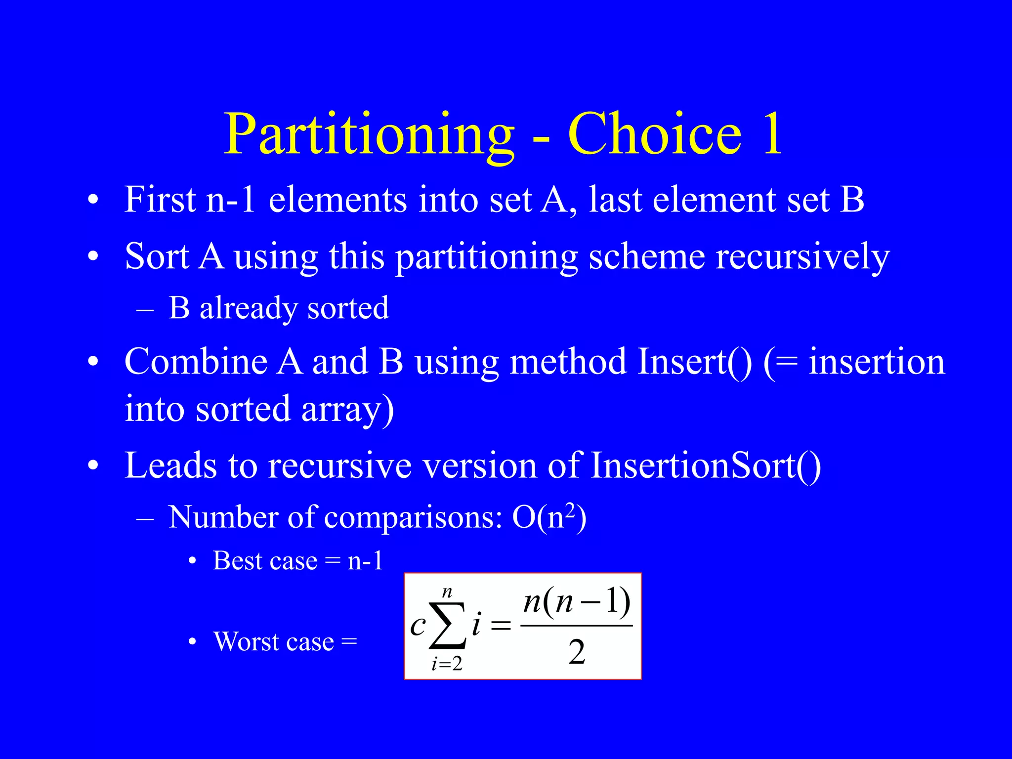
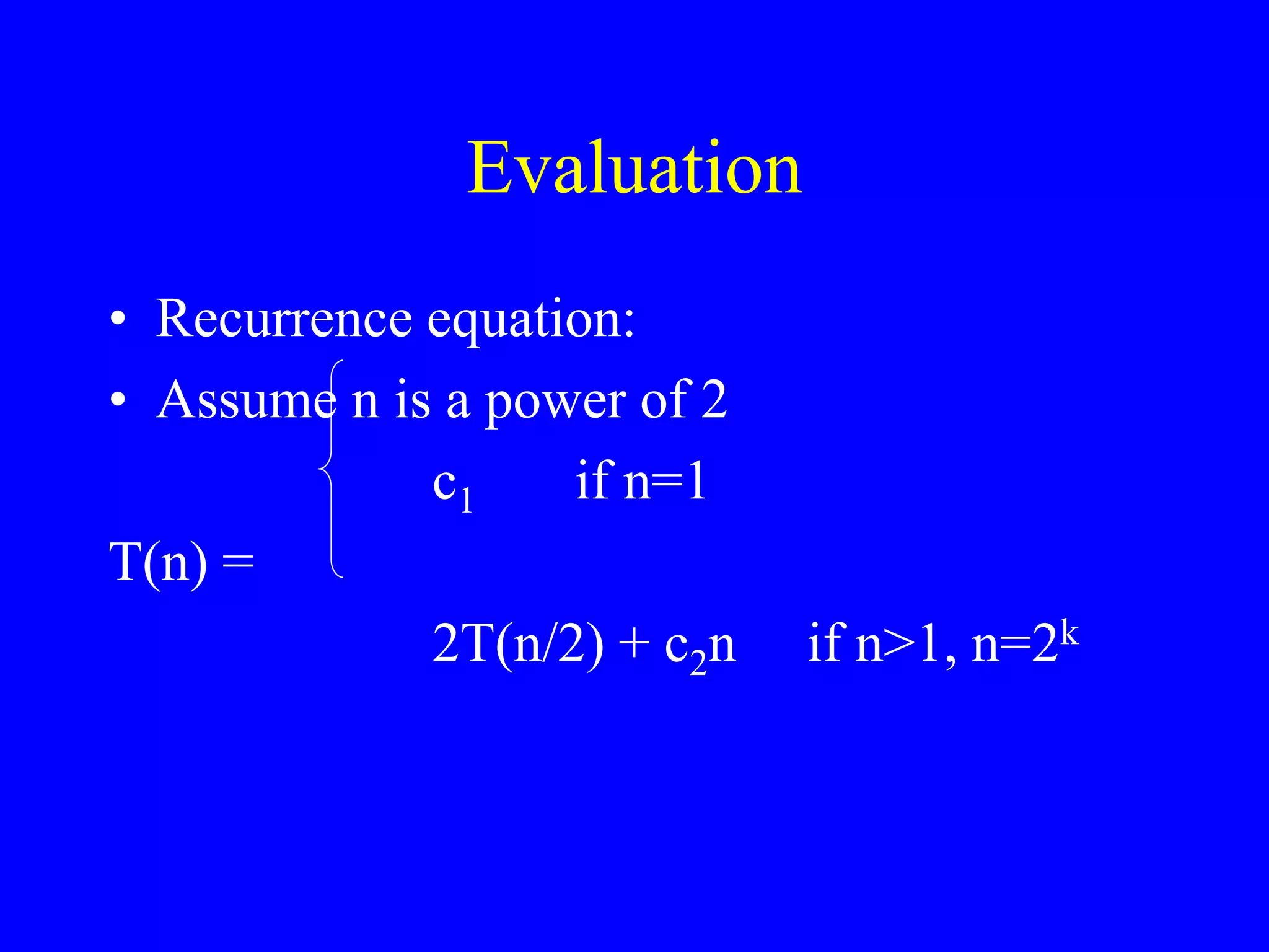
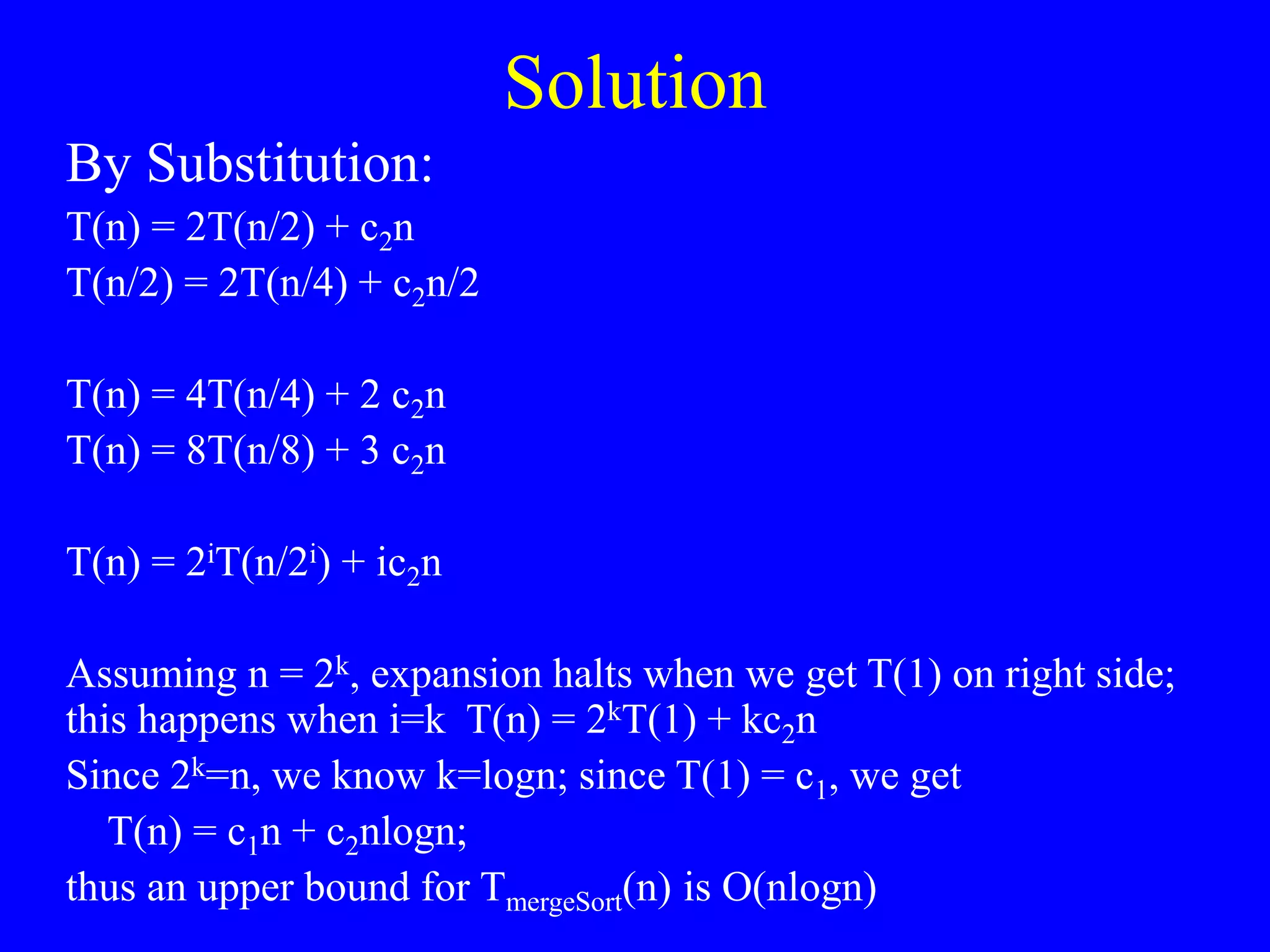
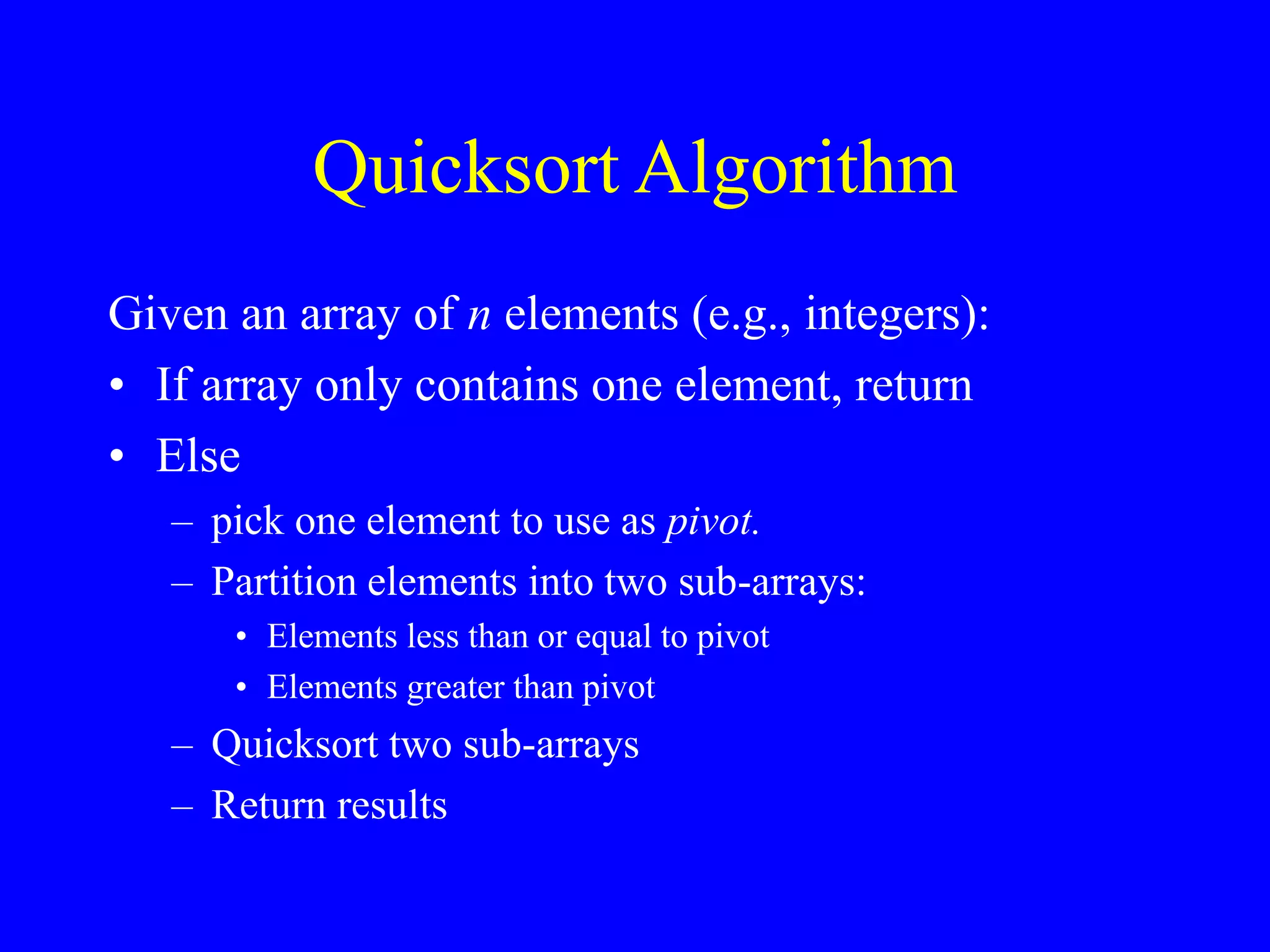
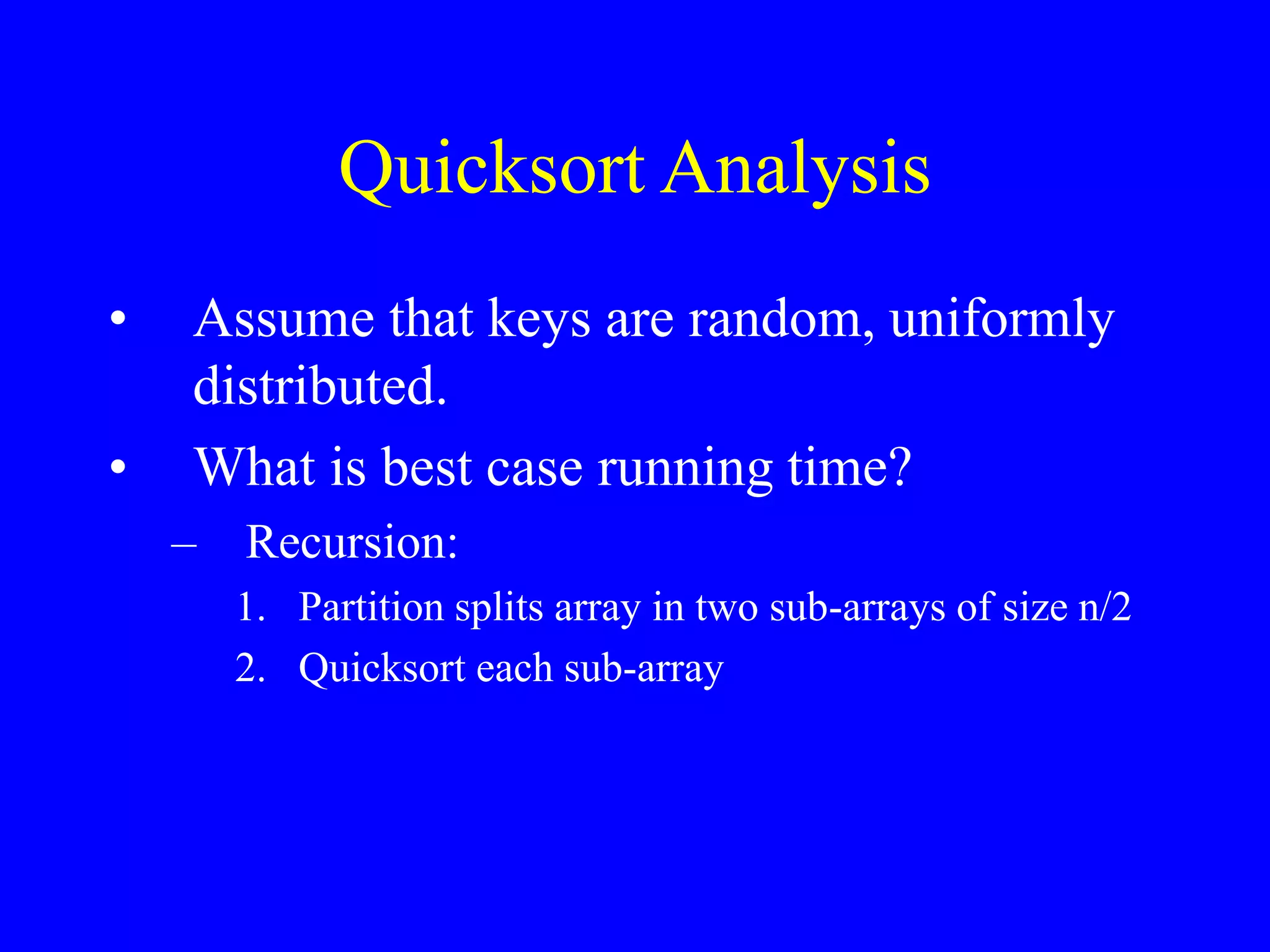
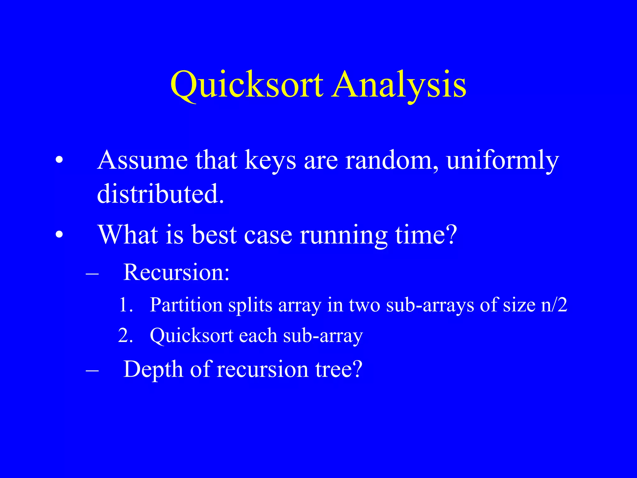
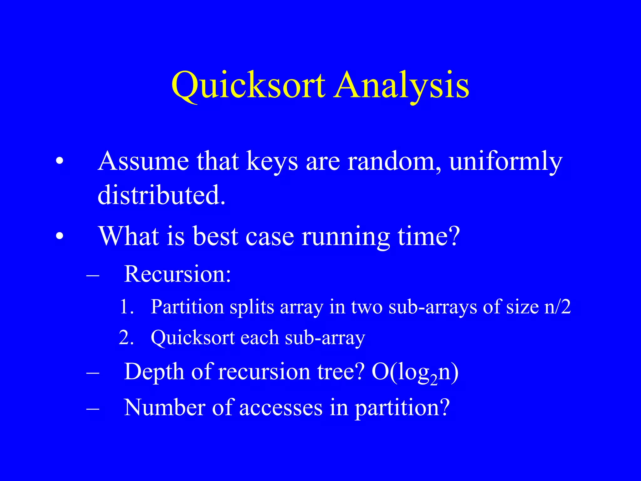
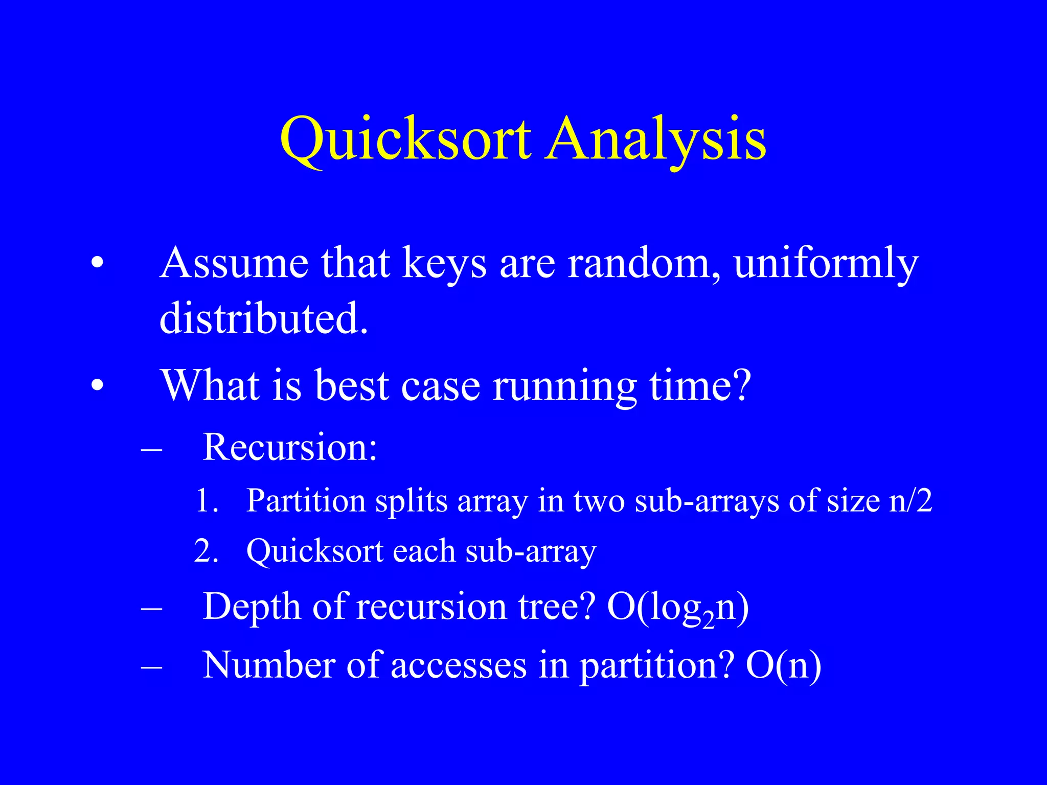
Mergesort and Quicksort are two efficient sorting algorithms that run in O(n log n) time. Mergesort uses a divide-and-conquer approach, recursively splitting the list into halves until individual elements remain, then merging the sorted halves back together. Quicksort chooses a pivot element and partitions the list into elements less than or greater than the pivot, then recursively sorts the sublists until the entire list is sorted.


![Example
• Partition into lists of size n/2
[10, 4, 6, 3]
[10, 4, 6, 3, 8, 2, 5, 7]
[8, 2, 5, 7]
[10, 4] [6, 3] [8, 2] [5, 7]
[4] [10] [3][6] [2][8] [5][7]](https://image.slidesharecdn.com/quickmergesort-230531094443-11a0d49b/75/Quick-Merge-Sort-ppt-7-2048.jpg)
![Example Cont’d
• Merge
[3, 4, 6, 10]
[2, 3, 4, 5, 6, 7, 8, 10 ]
[2, 5, 7, 8]
[4, 10] [3, 6] [2, 8] [5, 7]
[4] [10] [3][6] [2][8] [5][7]](https://image.slidesharecdn.com/quickmergesort-230531094443-11a0d49b/75/Quick-Merge-Sort-ppt-8-2048.jpg)
![Static Method mergeSort()
Public static void mergeSort(Comparable []a, int left,
int right)
{
// sort a[left:right]
if (left < right)
{// at least two elements
int mid = (left+right)/2; //midpoint
mergeSort(a, left, mid);
mergeSort(a, mid + 1, right);
merge(a, b, left, mid, right); //merge from a to b
copy(b, a, left, right); //copy result back to a
}
}](https://image.slidesharecdn.com/quickmergesort-230531094443-11a0d49b/75/Quick-Merge-Sort-ppt-9-2048.jpg)

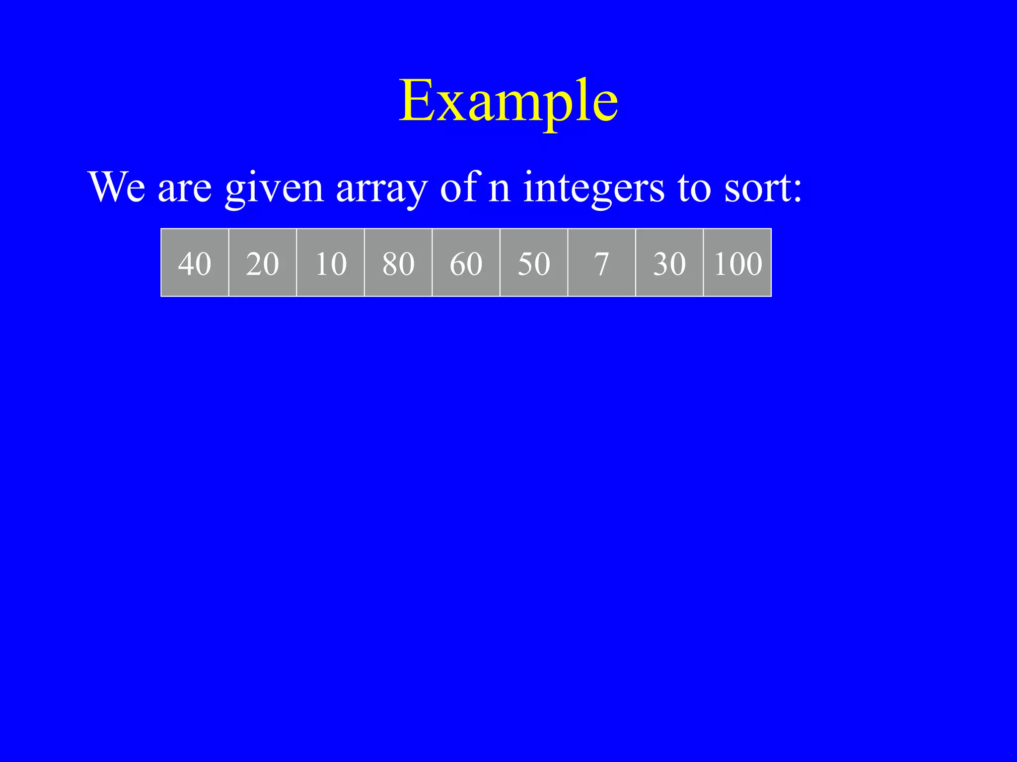

![40 20 10 80 60 50 7 30 100
pivot_index = 0
[0] [1] [2] [3] [4] [5] [6] [7] [8]
too_big_index too_small_index](https://image.slidesharecdn.com/quickmergesort-230531094443-11a0d49b/75/Quick-Merge-Sort-ppt-17-2048.jpg)
![40 20 10 80 60 50 7 30 100
pivot_index = 0
[0] [1] [2] [3] [4] [5] [6] [7] [8]
too_big_index too_small_index
1. While data[too_big_index] <= data[pivot]
++too_big_index](https://image.slidesharecdn.com/quickmergesort-230531094443-11a0d49b/75/Quick-Merge-Sort-ppt-18-2048.jpg)
![40 20 10 80 60 50 7 30 100
pivot_index = 0
[0] [1] [2] [3] [4] [5] [6] [7] [8]
too_big_index too_small_index
1. While data[too_big_index] <= data[pivot]
++too_big_index](https://image.slidesharecdn.com/quickmergesort-230531094443-11a0d49b/75/Quick-Merge-Sort-ppt-19-2048.jpg)
![40 20 10 80 60 50 7 30 100
pivot_index = 0
[0] [1] [2] [3] [4] [5] [6] [7] [8]
too_big_index too_small_index
1. While data[too_big_index] <= data[pivot]
++too_big_index](https://image.slidesharecdn.com/quickmergesort-230531094443-11a0d49b/75/Quick-Merge-Sort-ppt-20-2048.jpg)
![40 20 10 80 60 50 7 30 100
pivot_index = 0
[0] [1] [2] [3] [4] [5] [6] [7] [8]
too_big_index too_small_index
1. While data[too_big_index] <= data[pivot]
++too_big_index
2. While data[too_small_index] > data[pivot]
--too_small_index](https://image.slidesharecdn.com/quickmergesort-230531094443-11a0d49b/75/Quick-Merge-Sort-ppt-21-2048.jpg)
![40 20 10 80 60 50 7 30 100
pivot_index = 0
[0] [1] [2] [3] [4] [5] [6] [7] [8]
too_big_index too_small_index
1. While data[too_big_index] <= data[pivot]
++too_big_index
2. While data[too_small_index] > data[pivot]
--too_small_index](https://image.slidesharecdn.com/quickmergesort-230531094443-11a0d49b/75/Quick-Merge-Sort-ppt-22-2048.jpg)
![40 20 10 80 60 50 7 30 100
pivot_index = 0
[0] [1] [2] [3] [4] [5] [6] [7] [8]
too_big_index too_small_index
1. While data[too_big_index] <= data[pivot]
++too_big_index
2. While data[too_small_index] > data[pivot]
--too_small_index
3. If too_big_index < too_small_index
swap data[too_big_index] and data[too_small_index]](https://image.slidesharecdn.com/quickmergesort-230531094443-11a0d49b/75/Quick-Merge-Sort-ppt-23-2048.jpg)
![40 20 10 30 60 50 7 80 100
pivot_index = 0
[0] [1] [2] [3] [4] [5] [6] [7] [8]
too_big_index too_small_index
1. While data[too_big_index] <= data[pivot]
++too_big_index
2. While data[too_small_index] > data[pivot]
--too_small_index
3. If too_big_index < too_small_index
swap data[too_big_index] and data[too_small_index]](https://image.slidesharecdn.com/quickmergesort-230531094443-11a0d49b/75/Quick-Merge-Sort-ppt-24-2048.jpg)
![40 20 10 30 60 50 7 80 100
pivot_index = 0
[0] [1] [2] [3] [4] [5] [6] [7] [8]
too_big_index too_small_index
1. While data[too_big_index] <= data[pivot]
++too_big_index
2. While data[too_small_index] > data[pivot]
--too_small_index
3. If too_big_index < too_small_index
swap data[too_big_index] and data[too_small_index]
4. While too_small_index > too_big_index, go to 1.](https://image.slidesharecdn.com/quickmergesort-230531094443-11a0d49b/75/Quick-Merge-Sort-ppt-25-2048.jpg)
![40 20 10 30 60 50 7 80 100
pivot_index = 0
[0] [1] [2] [3] [4] [5] [6] [7] [8]
too_big_index too_small_index
1. While data[too_big_index] <= data[pivot]
++too_big_index
2. While data[too_small_index] > data[pivot]
--too_small_index
3. If too_big_index < too_small_index
swap data[too_big_index] and data[too_small_index]
4. While too_small_index > too_big_index, go to 1.](https://image.slidesharecdn.com/quickmergesort-230531094443-11a0d49b/75/Quick-Merge-Sort-ppt-26-2048.jpg)
![40 20 10 30 60 50 7 80 100
pivot_index = 0
[0] [1] [2] [3] [4] [5] [6] [7] [8]
too_big_index too_small_index
1. While data[too_big_index] <= data[pivot]
++too_big_index
2. While data[too_small_index] > data[pivot]
--too_small_index
3. If too_big_index < too_small_index
swap data[too_big_index] and data[too_small_index]
4. While too_small_index > too_big_index, go to 1.](https://image.slidesharecdn.com/quickmergesort-230531094443-11a0d49b/75/Quick-Merge-Sort-ppt-27-2048.jpg)
![40 20 10 30 60 50 7 80 100
pivot_index = 0
[0] [1] [2] [3] [4] [5] [6] [7] [8]
too_big_index too_small_index
1. While data[too_big_index] <= data[pivot]
++too_big_index
2. While data[too_small_index] > data[pivot]
--too_small_index
3. If too_big_index < too_small_index
swap data[too_big_index] and data[too_small_index]
4. While too_small_index > too_big_index, go to 1.](https://image.slidesharecdn.com/quickmergesort-230531094443-11a0d49b/75/Quick-Merge-Sort-ppt-28-2048.jpg)
![40 20 10 30 60 50 7 80 100
pivot_index = 0
[0] [1] [2] [3] [4] [5] [6] [7] [8]
too_big_index too_small_index
1. While data[too_big_index] <= data[pivot]
++too_big_index
2. While data[too_small_index] > data[pivot]
--too_small_index
3. If too_big_index < too_small_index
swap data[too_big_index] and data[too_small_index]
4. While too_small_index > too_big_index, go to 1.](https://image.slidesharecdn.com/quickmergesort-230531094443-11a0d49b/75/Quick-Merge-Sort-ppt-29-2048.jpg)
![40 20 10 30 60 50 7 80 100
pivot_index = 0
[0] [1] [2] [3] [4] [5] [6] [7] [8]
too_big_index too_small_index
1. While data[too_big_index] <= data[pivot]
++too_big_index
2. While data[too_small_index] > data[pivot]
--too_small_index
3. If too_big_index < too_small_index
swap data[too_big_index] and data[too_small_index]
4. While too_small_index > too_big_index, go to 1.](https://image.slidesharecdn.com/quickmergesort-230531094443-11a0d49b/75/Quick-Merge-Sort-ppt-30-2048.jpg)
![1. While data[too_big_index] <= data[pivot]
++too_big_index
2. While data[too_small_index] > data[pivot]
--too_small_index
3. If too_big_index < too_small_index
swap data[too_big_index] and data[too_small_index]
4. While too_small_index > too_big_index, go to 1.
40 20 10 30 7 50 60 80 100
pivot_index = 0
[0] [1] [2] [3] [4] [5] [6] [7] [8]
too_big_index too_small_index](https://image.slidesharecdn.com/quickmergesort-230531094443-11a0d49b/75/Quick-Merge-Sort-ppt-31-2048.jpg)
![1. While data[too_big_index] <= data[pivot]
++too_big_index
2. While data[too_small_index] > data[pivot]
--too_small_index
3. If too_big_index < too_small_index
swap data[too_big_index] and data[too_small_index]
4. While too_small_index > too_big_index, go to 1.
40 20 10 30 7 50 60 80 100
pivot_index = 0
[0] [1] [2] [3] [4] [5] [6] [7] [8]
too_big_index too_small_index](https://image.slidesharecdn.com/quickmergesort-230531094443-11a0d49b/75/Quick-Merge-Sort-ppt-32-2048.jpg)
![1. While data[too_big_index] <= data[pivot]
++too_big_index
2. While data[too_small_index] > data[pivot]
--too_small_index
3. If too_big_index < too_small_index
swap data[too_big_index] and data[too_small_index]
4. While too_small_index > too_big_index, go to 1.
40 20 10 30 7 50 60 80 100
pivot_index = 0
[0] [1] [2] [3] [4] [5] [6] [7] [8]
too_big_index too_small_index](https://image.slidesharecdn.com/quickmergesort-230531094443-11a0d49b/75/Quick-Merge-Sort-ppt-33-2048.jpg)
![1. While data[too_big_index] <= data[pivot]
++too_big_index
2. While data[too_small_index] > data[pivot]
--too_small_index
3. If too_big_index < too_small_index
swap data[too_big_index] and data[too_small_index]
4. While too_small_index > too_big_index, go to 1.
40 20 10 30 7 50 60 80 100
pivot_index = 0
[0] [1] [2] [3] [4] [5] [6] [7] [8]
too_big_index too_small_index](https://image.slidesharecdn.com/quickmergesort-230531094443-11a0d49b/75/Quick-Merge-Sort-ppt-34-2048.jpg)
![1. While data[too_big_index] <= data[pivot]
++too_big_index
2. While data[too_small_index] > data[pivot]
--too_small_index
3. If too_big_index < too_small_index
swap data[too_big_index] and data[too_small_index]
4. While too_small_index > too_big_index, go to 1.
40 20 10 30 7 50 60 80 100
pivot_index = 0
[0] [1] [2] [3] [4] [5] [6] [7] [8]
too_big_index too_small_index](https://image.slidesharecdn.com/quickmergesort-230531094443-11a0d49b/75/Quick-Merge-Sort-ppt-35-2048.jpg)
![1. While data[too_big_index] <= data[pivot]
++too_big_index
2. While data[too_small_index] > data[pivot]
--too_small_index
3. If too_big_index < too_small_index
swap data[too_big_index] and data[too_small_index]
4. While too_small_index > too_big_index, go to 1.
40 20 10 30 7 50 60 80 100
pivot_index = 0
[0] [1] [2] [3] [4] [5] [6] [7] [8]
too_big_index too_small_index](https://image.slidesharecdn.com/quickmergesort-230531094443-11a0d49b/75/Quick-Merge-Sort-ppt-36-2048.jpg)
![1. While data[too_big_index] <= data[pivot]
++too_big_index
2. While data[too_small_index] > data[pivot]
--too_small_index
3. If too_big_index < too_small_index
swap data[too_big_index] and data[too_small_index]
4. While too_small_index > too_big_index, go to 1.
40 20 10 30 7 50 60 80 100
pivot_index = 0
[0] [1] [2] [3] [4] [5] [6] [7] [8]
too_big_index too_small_index](https://image.slidesharecdn.com/quickmergesort-230531094443-11a0d49b/75/Quick-Merge-Sort-ppt-37-2048.jpg)
![1. While data[too_big_index] <= data[pivot]
++too_big_index
2. While data[too_small_index] > data[pivot]
--too_small_index
3. If too_big_index < too_small_index
swap data[too_big_index] and data[too_small_index]
4. While too_small_index > too_big_index, go to 1.
40 20 10 30 7 50 60 80 100
pivot_index = 0
[0] [1] [2] [3] [4] [5] [6] [7] [8]
too_big_index too_small_index](https://image.slidesharecdn.com/quickmergesort-230531094443-11a0d49b/75/Quick-Merge-Sort-ppt-38-2048.jpg)
![1. While data[too_big_index] <= data[pivot]
++too_big_index
2. While data[too_small_index] > data[pivot]
--too_small_index
3. If too_big_index < too_small_index
swap data[too_big_index] and data[too_small_index]
4. While too_small_index > too_big_index, go to 1.
40 20 10 30 7 50 60 80 100
pivot_index = 0
[0] [1] [2] [3] [4] [5] [6] [7] [8]
too_big_index too_small_index](https://image.slidesharecdn.com/quickmergesort-230531094443-11a0d49b/75/Quick-Merge-Sort-ppt-39-2048.jpg)
![1. While data[too_big_index] <= data[pivot]
++too_big_index
2. While data[too_small_index] > data[pivot]
--too_small_index
3. If too_big_index < too_small_index
swap data[too_big_index] and data[too_small_index]
4. While too_small_index > too_big_index, go to 1.
5. Swap data[too_small_index] and data[pivot_index]
40 20 10 30 7 50 60 80 100
pivot_index = 0
[0] [1] [2] [3] [4] [5] [6] [7] [8]
too_big_index too_small_index](https://image.slidesharecdn.com/quickmergesort-230531094443-11a0d49b/75/Quick-Merge-Sort-ppt-40-2048.jpg)
![1. While data[too_big_index] <= data[pivot]
++too_big_index
2. While data[too_small_index] > data[pivot]
--too_small_index
3. If too_big_index < too_small_index
swap data[too_big_index] and data[too_small_index]
4. While too_small_index > too_big_index, go to 1.
5. Swap data[too_small_index] and data[pivot_index]
7 20 10 30 40 50 60 80 100
pivot_index = 4
[0] [1] [2] [3] [4] [5] [6] [7] [8]
too_big_index too_small_index](https://image.slidesharecdn.com/quickmergesort-230531094443-11a0d49b/75/Quick-Merge-Sort-ppt-41-2048.jpg)
![Partition Result
7 20 10 30 40 50 60 80 100
[0] [1] [2] [3] [4] [5] [6] [7] [8]
<= data[pivot] > data[pivot]](https://image.slidesharecdn.com/quickmergesort-230531094443-11a0d49b/75/Quick-Merge-Sort-ppt-42-2048.jpg)
![Recursion: Quicksort Sub-arrays
7 20 10 30 40 50 60 80 100
[0] [1] [2] [3] [4] [5] [6] [7] [8]
<= data[pivot] > data[pivot]](https://image.slidesharecdn.com/quickmergesort-230531094443-11a0d49b/75/Quick-Merge-Sort-ppt-43-2048.jpg)

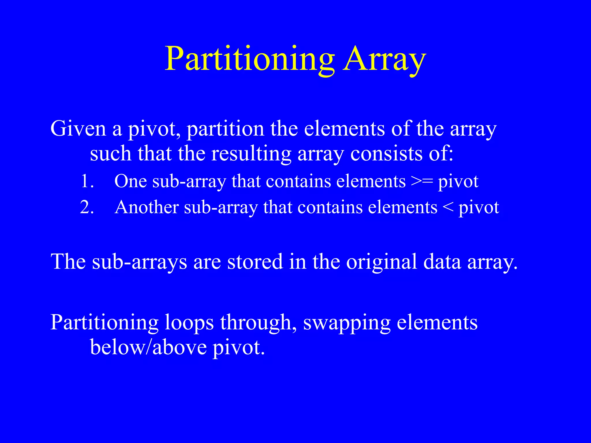
![Quicksort: Worst Case
• Assume first element is chosen as pivot.
• Assume we get array that is already in
order:
2 4 10 12 13 50 57 63 100
pivot_index = 0
[0] [1] [2] [3] [4] [5] [6] [7] [8]
too_big_index too_small_index](https://image.slidesharecdn.com/quickmergesort-230531094443-11a0d49b/75/Quick-Merge-Sort-ppt-52-2048.jpg)
![1. While data[too_big_index] <= data[pivot]
++too_big_index
2. While data[too_small_index] > data[pivot]
--too_small_index
3. If too_big_index < too_small_index
swap data[too_big_index] and data[too_small_index]
4. While too_small_index > too_big_index, go to 1.
5. Swap data[too_small_index] and data[pivot_index]
2 4 10 12 13 50 57 63 100
pivot_index = 0
[0] [1] [2] [3] [4] [5] [6] [7] [8]
too_big_index too_small_index](https://image.slidesharecdn.com/quickmergesort-230531094443-11a0d49b/75/Quick-Merge-Sort-ppt-53-2048.jpg)
![1. While data[too_big_index] <= data[pivot]
++too_big_index
2. While data[too_small_index] > data[pivot]
--too_small_index
3. If too_big_index < too_small_index
swap data[too_big_index] and data[too_small_index]
4. While too_small_index > too_big_index, go to 1.
5. Swap data[too_small_index] and data[pivot_index]
2 4 10 12 13 50 57 63 100
pivot_index = 0
[0] [1] [2] [3] [4] [5] [6] [7] [8]
too_big_index too_small_index](https://image.slidesharecdn.com/quickmergesort-230531094443-11a0d49b/75/Quick-Merge-Sort-ppt-54-2048.jpg)
![1. While data[too_big_index] <= data[pivot]
++too_big_index
2. While data[too_small_index] > data[pivot]
--too_small_index
3. If too_big_index < too_small_index
swap data[too_big_index] and data[too_small_index]
4. While too_small_index > too_big_index, go to 1.
5. Swap data[too_small_index] and data[pivot_index]
2 4 10 12 13 50 57 63 100
pivot_index = 0
[0] [1] [2] [3] [4] [5] [6] [7] [8]
too_big_index too_small_index](https://image.slidesharecdn.com/quickmergesort-230531094443-11a0d49b/75/Quick-Merge-Sort-ppt-55-2048.jpg)
![1. While data[too_big_index] <= data[pivot]
++too_big_index
2. While data[too_small_index] > data[pivot]
--too_small_index
3. If too_big_index < too_small_index
swap data[too_big_index] and data[too_small_index]
4. While too_small_index > too_big_index, go to 1.
5. Swap data[too_small_index] and data[pivot_index]
2 4 10 12 13 50 57 63 100
pivot_index = 0
[0] [1] [2] [3] [4] [5] [6] [7] [8]
too_big_index too_small_index](https://image.slidesharecdn.com/quickmergesort-230531094443-11a0d49b/75/Quick-Merge-Sort-ppt-56-2048.jpg)
![1. While data[too_big_index] <= data[pivot]
++too_big_index
2. While data[too_small_index] > data[pivot]
--too_small_index
3. If too_big_index < too_small_index
swap data[too_big_index] and data[too_small_index]
4. While too_small_index > too_big_index, go to 1.
5. Swap data[too_small_index] and data[pivot_index]
2 4 10 12 13 50 57 63 100
pivot_index = 0
[0] [1] [2] [3] [4] [5] [6] [7] [8]
too_big_index too_small_index](https://image.slidesharecdn.com/quickmergesort-230531094443-11a0d49b/75/Quick-Merge-Sort-ppt-57-2048.jpg)
![1. While data[too_big_index] <= data[pivot]
++too_big_index
2. While data[too_small_index] > data[pivot]
--too_small_index
3. If too_big_index < too_small_index
swap data[too_big_index] and data[too_small_index]
4. While too_small_index > too_big_index, go to 1.
5. Swap data[too_small_index] and data[pivot_index]
2 4 10 12 13 50 57 63 100
pivot_index = 0
[0] [1] [2] [3] [4] [5] [6] [7] [8]
too_big_index too_small_index](https://image.slidesharecdn.com/quickmergesort-230531094443-11a0d49b/75/Quick-Merge-Sort-ppt-58-2048.jpg)
![1. While data[too_big_index] <= data[pivot]
++too_big_index
2. While data[too_small_index] > data[pivot]
--too_small_index
3. If too_big_index < too_small_index
swap data[too_big_index] and data[too_small_index]
4. While too_small_index > too_big_index, go to 1.
5. Swap data[too_small_index] and data[pivot_index]
2 4 10 12 13 50 57 63 100
pivot_index = 0
[0] [1] [2] [3] [4] [5] [6] [7] [8]
> data[pivot]
<= data[pivot]](https://image.slidesharecdn.com/quickmergesort-230531094443-11a0d49b/75/Quick-Merge-Sort-ppt-59-2048.jpg)
![Improved Pivot Selection
Pick median value of three elements from data array:
data[0], data[n/2], and data[n-1].
Use this median value as pivot.](https://image.slidesharecdn.com/quickmergesort-230531094443-11a0d49b/75/Quick-Merge-Sort-ppt-66-2048.jpg)
![Improving Performance of
Quicksort
• Improved selection of pivot.
• For sub-arrays of size 3 or less, apply brute
force search:
– Sub-array of size 1: trivial
– Sub-array of size 2:
• if(data[first] > data[second]) swap them
– Sub-array of size 3: left as an exercise.](https://image.slidesharecdn.com/quickmergesort-230531094443-11a0d49b/75/Quick-Merge-Sort-ppt-67-2048.jpg)