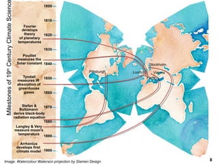
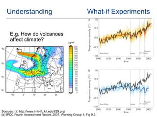
Modeling the Climate System:
Is model-based science like model-based engineering?
Steve Easterbrook
Email: sme@cs.toronto.edu
Blog: www.easterbrook.ca/steve
Twitter: @SMEasterbrook
2
Climate Modeling vs S/W Engineering
Continuous math
E.g. partial differential
equations
Models of
“How things are”
Discrete math
E.g. state machines,
graphs, FOL
Models of
“How things should be”
Modeling as a strategy for testing our ideas about
the world when direct experimentation isn’t possible.
Modeling to support collaboration and
communication in a diverse community of practice.
Modeling to support wise decision-making about our
future course of action.
Modeling as a strategy for testing our ideas about
the world when direct experimentation isn’t possible.
Modeling to support collaboration and
communication in a diverse community of practice.
Modeling to support wise decision-making about our
future course of action.
3
Outline
1. What are climate models?
In which we step back in time and meet a 19th Century Swedish chemist
and a famous computer scientist.
1. How are they used?
In which we perform two dangerous experiments on the life support systems
of planet earth but live to tell the tale.
1. What are the engineering challenges?
In which we share war stories about the difficulties of model management in
the real world.
1. Conclusion: So how is climate modeling like software
modeling?
In which I wave my arms a lot.
4
5
Complex software systems…
Easterbrook, S. M., & Johns, T. C. (2009). Engineering the Software for Understanding
Climate Change. Computing in Science and Engineering, 11(6), 65–74.
Easterbrook, S. M., & Johns, T. C. (2009). Engineering the Software for Understanding
Climate Change. Computing in Science and Engineering, 11(6), 65–74.
6
Alexander, K., Easterbrook, S. (2015). The software architecture of climate models: a graphical
comparison of CMIP5 and EMICAR5 configurations. Geoscientific Model Development 8, 1221-1232.
Alexander, K., Easterbrook, S. (2015). The software architecture of climate models: a graphical
comparison of CMIP5 and EMICAR5 configurations. Geoscientific Model Development 8, 1221-1232.
Complex software eco-systems…
7
The First Computational Climate Model
1895: Svante Arrhenius constructs an energy balance model to test his
hypothesis that the ice ages were caused by a drop in CO2;
(Predicts global temperature rise of 5.7°C if we double CO2)
Stockholm
8
Pittsburgh
Stockholm
Paris
London
Milestonesof19th
CenturyClimateScienc
Vienna
Image: Watercolour Waterson projection by Stamen Design
9Image Source: https://chriscolose.wordpress.com/2010/02/18/greenhouse-effect-revisited/
Warm objects radiate infra-red
10Image Source: http://rabett.blogspot.ca/2010/03/simplest-explanation.html
Absorption fingerprint of greenhouse gases
In some wavelength bands, the atmosphere is
transparent to infra-red. Emissions to space
are from the (warmer) ground
In bands where greenhouse gases block infra-red
from the ground, emissions to space come from
the (cooler) upper atmosphere
11
Schematic of the model equations
12
Arrhenius’s Model Outputs
Image Source: Arrhenius, S. (1896). On the Influence of Carbonic Acid in the Air upon the Temperature of the Ground.
13
First Computer Model of Weather
1950s: John Von Neumann develops a killer app for the first
programmable electronic computer ENIAC: weather forecasting
Imagines uses in weather control, geo-engineering, etc.
14Image Source: Lynch, P. (2008). The ENIAC Forecasts: A Recreation. Bulletin of the American Meteorological Society
15
Basic physical equations
Zonal (East-West) Wind:
Meridional (North-South) Wind:
Temperature:
Precipitable Water:
Air pressure:
1904: Vilhelm Bjerknes identified the “primitive equations”
These capture the flow of mass and energy in the atmosphere;
Sets out a manifesto for practical forecasting
16
Towards Numerical Forecasts
1910s: Lewis Fry Richardson performs the first numerical weather
forecast, imagines a giant computer to do this regularly;
First plan for massively parallel computation
Image Source: Lynch, P. (2008). The origins of computer weather prediction and climate modeling.
17
(What a forecast factory actually looks like)
The Yellowstone supercomputer at the NCAR Wyoming Supercomputing Center, Cheyenne
18
Towards Earth System Models
Atmosphere Atmosphere Atmosphere Atmosphere Atmosphere Atmosphere
Land surface
+ land ice?Land surfaceLand surfaceLand surfaceLand surface
Ocean & sea-ice Ocean & sea-ice Ocean & sea-ice
New
Ocean & sea-ice
Sulphate
aerosol
Sulphate
aerosol
Sulphate
aerosol
Non-sulphate
aerosol
Non-sulphate
aerosol
Carbon
(+ N?) cycle
Atmospheric
chemistry
Ocean & sea-ice
model
Sulphur
cycle model
Non-sulphate
aerosols
Carbon
cycle model
Land carbon
cycle model
Ocean carbon
cycle model
Atmospheric
chemistry
Atmospheric
chemistry
Off-line
model
development
Strengthening colours
denote improvements
in models
1975 1985 1992 1997 2004/05 2009/11
HadCM3 HadGEM1 HadGEM2
Image:UKMetOffice©CrownCopyright
19Image Source: IPCC Fifth Assessment Report, Jan 2014. Working Group 1, Fig 1.14(b)
Grid scale in a high resolution model
20
From: Knutti, R., & Sedláček, J. (2012). Robustness and uncertainties in the new CMIP5 climate model projections. Nature Climate
Change, (October), 1–5.
21
Can we limit warming to >+2ºC?
From: MR Allen et al. Nature 458, 1163-1166 (2009)
22
Can we artificially cool the planet?
From: Berdahl, M., et al. (2014). Arctic cryosphere response in the Geoengineering Model Intercomparison
Project G3 and G4 scenarios. Journal of Geophysical Research: Atmospheres, 119(3), 1308–1321.
Globalaveragenear-
surfacetemperature(°C)
ArticSeaIceExtent
(millionsofkm2
)
23
Some Observations
1) A model is never complete…
…but is sometimes good enough
24
?Model
Weakness
Develop
Hypothesis
Run
Experime
nt
Interpret
Results
Peer
Review
Try another hypothesis
OK
?
New Model
Version
Model building is “doing science”
25
Some Observations
2) Models are for testing and improving our
understanding of the world
(e.g. for “what-if” experiments)
26
Understanding What-if Experiments
E.g. How do volcanoes
affect climate?
Sources: (a) http://www.imk-ifu.kit.edu/829.php
(b) IPCC Fourth Assessment Report, 2007. Working Group 1, Fig 9.5.
27
Some Observations
3) Models enable communication and collaboration
28
Inter-disciplinary work is hard!
29
Coupled model
Atmospheric Dynamics
and Physics
Ocean Dynamics
Sea Ice
Land Surface
Processes
Atmospheric
Chemistry
Ocean
Biogeochemistry
Overlapping Communities
30
Some Observations
(A corollary)
4) Model Integration is inevitable
…unfortunately, it’s never easy
31
Example: NCAR, Boulder
Alexander, K., Easterbrook, S. (2015). The software architecture of climate models: a graphical
comparison of CMIP5 and EMICAR5 configurations. Geoscientific Model Development 8, 1221-1232.
Alexander, K., Easterbrook, S. (2015). The software architecture of climate models: a graphical
comparison of CMIP5 and EMICAR5 configurations. Geoscientific Model Development 8, 1221-1232.
32
Some Observations
5) A solitary model has very little value
33
Comparing multiple models
Model
Hierarchies
Multi-Model
Ensembles
Multiple
Versions
Sources: (a) Knutti, R. et al. (2013). Climate model genealogy: Generation CMIP5 and how we got there.
(b) http://efdl.as.ntu.edu.tw/research/timcom/
34
Some Observations
6) When the model and the world disagree, the
model is often right…
35
Observational data is often wrong
Thompson, D. W. J., Kennedy, J. J., Wallace, J. M., & Jones, P. D. (2008). A large discontinuity in the mid-twentieth century in
observed global-mean surface temperature. Nature, 453(7195), 646–649.
36
Some Observations
7 Complex models have emergent phenomena
…and when the model surprises you,
learning happens
37Source: http://www.vets.ucar.edu/vg/T341/index.shtml
Global Precipitation in CCSM CAM3
38
Some Observations
8) Most of what we need to know to interpret a
model’s output isn’t in the model itself…
39
A Climate
Model
Configuration
?
Scientific
Question
Model
Development,
Selection &
Configuration
Running
Model
Interpretation
of results
Papers &
Reports
Scope of typical
model evaluations
Scope of fitness-for-purpose
validation of a modeling system
Is this model configuration
appropriate to the
question?
Are the model outputs
used appropriately?
From models to modeling systems
40
Summary
1. A model is never complete, but is sometimes good enough
2. Models are for improving our understanding and asking
“what-if” questions.
3. Models enable close cross-disciplinary collaboration.
4. Model integration is difficult and inevitable.
5. A solitary model has very little value.
6. When the model and the data disagree, it’s often the data
that are wrong.
7. Complex models have emergent phenomena…
…and a model is most valuable when it surprises you
8. A model won’t make sense out of context
41Image: https://www.flickr.com/photos/good_day/211972522/

Modeling the Climate System: Is model-based science like model-based engineering?

  • 1.
    Modeling the ClimateSystem: Is model-based science like model-based engineering? Steve Easterbrook Email: sme@cs.toronto.edu Blog: www.easterbrook.ca/steve Twitter: @SMEasterbrook
  • 2.
    2 Climate Modeling vsS/W Engineering Continuous math E.g. partial differential equations Models of “How things are” Discrete math E.g. state machines, graphs, FOL Models of “How things should be” Modeling as a strategy for testing our ideas about the world when direct experimentation isn’t possible. Modeling to support collaboration and communication in a diverse community of practice. Modeling to support wise decision-making about our future course of action. Modeling as a strategy for testing our ideas about the world when direct experimentation isn’t possible. Modeling to support collaboration and communication in a diverse community of practice. Modeling to support wise decision-making about our future course of action.
  • 3.
    3 Outline 1. What areclimate models? In which we step back in time and meet a 19th Century Swedish chemist and a famous computer scientist. 1. How are they used? In which we perform two dangerous experiments on the life support systems of planet earth but live to tell the tale. 1. What are the engineering challenges? In which we share war stories about the difficulties of model management in the real world. 1. Conclusion: So how is climate modeling like software modeling? In which I wave my arms a lot.
  • 4.
  • 5.
    5 Complex software systems… Easterbrook,S. M., & Johns, T. C. (2009). Engineering the Software for Understanding Climate Change. Computing in Science and Engineering, 11(6), 65–74. Easterbrook, S. M., & Johns, T. C. (2009). Engineering the Software for Understanding Climate Change. Computing in Science and Engineering, 11(6), 65–74.
  • 6.
    6 Alexander, K., Easterbrook,S. (2015). The software architecture of climate models: a graphical comparison of CMIP5 and EMICAR5 configurations. Geoscientific Model Development 8, 1221-1232. Alexander, K., Easterbrook, S. (2015). The software architecture of climate models: a graphical comparison of CMIP5 and EMICAR5 configurations. Geoscientific Model Development 8, 1221-1232. Complex software eco-systems…
  • 7.
    7 The First ComputationalClimate Model 1895: Svante Arrhenius constructs an energy balance model to test his hypothesis that the ice ages were caused by a drop in CO2; (Predicts global temperature rise of 5.7°C if we double CO2) Stockholm
  • 8.
  • 9.
  • 10.
    10Image Source: http://rabett.blogspot.ca/2010/03/simplest-explanation.html Absorptionfingerprint of greenhouse gases In some wavelength bands, the atmosphere is transparent to infra-red. Emissions to space are from the (warmer) ground In bands where greenhouse gases block infra-red from the ground, emissions to space come from the (cooler) upper atmosphere
  • 11.
    11 Schematic of themodel equations
  • 12.
    12 Arrhenius’s Model Outputs ImageSource: Arrhenius, S. (1896). On the Influence of Carbonic Acid in the Air upon the Temperature of the Ground.
  • 13.
    13 First Computer Modelof Weather 1950s: John Von Neumann develops a killer app for the first programmable electronic computer ENIAC: weather forecasting Imagines uses in weather control, geo-engineering, etc.
  • 14.
    14Image Source: Lynch,P. (2008). The ENIAC Forecasts: A Recreation. Bulletin of the American Meteorological Society
  • 15.
    15 Basic physical equations Zonal(East-West) Wind: Meridional (North-South) Wind: Temperature: Precipitable Water: Air pressure: 1904: Vilhelm Bjerknes identified the “primitive equations” These capture the flow of mass and energy in the atmosphere; Sets out a manifesto for practical forecasting
  • 16.
    16 Towards Numerical Forecasts 1910s:Lewis Fry Richardson performs the first numerical weather forecast, imagines a giant computer to do this regularly; First plan for massively parallel computation Image Source: Lynch, P. (2008). The origins of computer weather prediction and climate modeling.
  • 17.
    17 (What a forecastfactory actually looks like) The Yellowstone supercomputer at the NCAR Wyoming Supercomputing Center, Cheyenne
  • 18.
    18 Towards Earth SystemModels Atmosphere Atmosphere Atmosphere Atmosphere Atmosphere Atmosphere Land surface + land ice?Land surfaceLand surfaceLand surfaceLand surface Ocean & sea-ice Ocean & sea-ice Ocean & sea-ice New Ocean & sea-ice Sulphate aerosol Sulphate aerosol Sulphate aerosol Non-sulphate aerosol Non-sulphate aerosol Carbon (+ N?) cycle Atmospheric chemistry Ocean & sea-ice model Sulphur cycle model Non-sulphate aerosols Carbon cycle model Land carbon cycle model Ocean carbon cycle model Atmospheric chemistry Atmospheric chemistry Off-line model development Strengthening colours denote improvements in models 1975 1985 1992 1997 2004/05 2009/11 HadCM3 HadGEM1 HadGEM2 Image:UKMetOffice©CrownCopyright
  • 19.
    19Image Source: IPCCFifth Assessment Report, Jan 2014. Working Group 1, Fig 1.14(b) Grid scale in a high resolution model
  • 20.
    20 From: Knutti, R.,& Sedláček, J. (2012). Robustness and uncertainties in the new CMIP5 climate model projections. Nature Climate Change, (October), 1–5.
  • 21.
    21 Can we limitwarming to >+2ºC? From: MR Allen et al. Nature 458, 1163-1166 (2009)
  • 22.
    22 Can we artificiallycool the planet? From: Berdahl, M., et al. (2014). Arctic cryosphere response in the Geoengineering Model Intercomparison Project G3 and G4 scenarios. Journal of Geophysical Research: Atmospheres, 119(3), 1308–1321. Globalaveragenear- surfacetemperature(°C) ArticSeaIceExtent (millionsofkm2 )
  • 23.
    23 Some Observations 1) Amodel is never complete… …but is sometimes good enough
  • 24.
  • 25.
    25 Some Observations 2) Modelsare for testing and improving our understanding of the world (e.g. for “what-if” experiments)
  • 26.
    26 Understanding What-if Experiments E.g.How do volcanoes affect climate? Sources: (a) http://www.imk-ifu.kit.edu/829.php (b) IPCC Fourth Assessment Report, 2007. Working Group 1, Fig 9.5.
  • 27.
    27 Some Observations 3) Modelsenable communication and collaboration
  • 28.
  • 29.
    29 Coupled model Atmospheric Dynamics andPhysics Ocean Dynamics Sea Ice Land Surface Processes Atmospheric Chemistry Ocean Biogeochemistry Overlapping Communities
  • 30.
    30 Some Observations (A corollary) 4)Model Integration is inevitable …unfortunately, it’s never easy
  • 31.
    31 Example: NCAR, Boulder Alexander,K., Easterbrook, S. (2015). The software architecture of climate models: a graphical comparison of CMIP5 and EMICAR5 configurations. Geoscientific Model Development 8, 1221-1232. Alexander, K., Easterbrook, S. (2015). The software architecture of climate models: a graphical comparison of CMIP5 and EMICAR5 configurations. Geoscientific Model Development 8, 1221-1232.
  • 32.
    32 Some Observations 5) Asolitary model has very little value
  • 33.
    33 Comparing multiple models Model Hierarchies Multi-Model Ensembles Multiple Versions Sources:(a) Knutti, R. et al. (2013). Climate model genealogy: Generation CMIP5 and how we got there. (b) http://efdl.as.ntu.edu.tw/research/timcom/
  • 34.
    34 Some Observations 6) Whenthe model and the world disagree, the model is often right…
  • 35.
    35 Observational data isoften wrong Thompson, D. W. J., Kennedy, J. J., Wallace, J. M., & Jones, P. D. (2008). A large discontinuity in the mid-twentieth century in observed global-mean surface temperature. Nature, 453(7195), 646–649.
  • 36.
    36 Some Observations 7 Complexmodels have emergent phenomena …and when the model surprises you, learning happens
  • 37.
  • 38.
    38 Some Observations 8) Mostof what we need to know to interpret a model’s output isn’t in the model itself…
  • 39.
    39 A Climate Model Configuration ? Scientific Question Model Development, Selection & Configuration Running Model Interpretation ofresults Papers & Reports Scope of typical model evaluations Scope of fitness-for-purpose validation of a modeling system Is this model configuration appropriate to the question? Are the model outputs used appropriately? From models to modeling systems
  • 40.
    40 Summary 1. A modelis never complete, but is sometimes good enough 2. Models are for improving our understanding and asking “what-if” questions. 3. Models enable close cross-disciplinary collaboration. 4. Model integration is difficult and inevitable. 5. A solitary model has very little value. 6. When the model and the data disagree, it’s often the data that are wrong. 7. Complex models have emergent phenomena… …and a model is most valuable when it surprises you 8. A model won’t make sense out of context
  • 41.

Editor's Notes

  • #5 Most of the observations in this talk come from a series of ethnographic studies of how climate scientists build climate models. I started these studies expecting to be able to help the climate modelers with better software engineering techniques. While some of the software engineering is very ad hoc, for the bigger models, the labs have developed a very disciplined software development process. There are some opportunities to adopt new tools and techniques, but many of the obvious candidate tools don’t readily apply. They use a highly tailored software development process that is highly embedded in their scientific methodology, and offers some interesting lessons for software engineering in general.
  • #6 Here are some indicators of that growth. This chart shows the growth of the UKMO Unified Model over the last fifteen years in terms of lines of code. The green line at the top is lines of code, while the blue line is number of files (roughly, Fortran Modules). Over a fifteen year period, the code base grew from 100,000 lines of code, to almost a million - an order of magnitude change. This analysis comes from the first study we published, back in 2009.
  • #7 Source code for the models is readily available.
  • #10 Total area under the curve corresponds to total energy emitted.
  • #13 Talk about the grid: he solves the equations for each grid point. Notes: No notion of time in this model; it’s a snapshot of the radiative physics at equilibrium. If you really want to know how the climate system works, you need to get the dynamics into the model.
  • #15 Lynch, P. (2008). The ENIAC Forecasts: A Recreation. Bulletin of the American Meteorological Society, (January), 1–11.
  • #16 Manifesto: Two steps: Diagnostic Step and a Prognostic Step. Primitive equations: A continuity equation, for conservation of mass Conservation of momentum – a form of the navier-stokes equations adapted to flow on a rotating sphere Thermal energy equation, to conserve energy within the system, taking into account sources and sinks.
  • #17 In the middle of his work as an ambulance driver on the front line in France during WW1, Richardson computed the first ever numerical forecast, calculating the change in wind and air pressure at two points, based on starting conditions on 20 May 2910. It probably took him about 2 years to compute, working say 10 hours per week. He got it wrong, but largely because of inaccuracies in the initial conditions. He calculated that 32 people working together could have done the calculation fast enough to keep up with the real weather. Furthermore, that was for just one grid point. He imagined dividing up the entire globe into 200km squares, needing about 2000 columns of air, and assigning 32 computers (people!!) to each, for a total of 64,000 people. He imagined them on balconies in a huge hollow sphere, with a conductor in the middle shining beams of light on those computers who were falling behind in their task.
  • #18 So I described two components: radiative physics of the greenhouse effect and dynamics of the atmosphere (and do the same for ocean). But models have evolved since then.
  • #21 This is the tip of the iceberg – the part of climate modeling that people (outside the modeling community see).
  • #22 Here’s the analysis from the paper. It’s a probablistic forecast, achieved by running a large ensemble of climate models - a multi-model ensemble. Using an ensemble of models from different labs has been shown to give better reproductions of past climates than just using a single model. The first graph shows some potential emissions pathways. The orange paths are those that stick within 1% of the 1 trillion tonne cumulative limit for the period 1750 to 2500. The solid red line is an example case, selected as a benchmark. The dotted red line represents a scenario that stabilizes concentrations at 490ppm. The middle graph shows the resulting CO2 concentration for (only) the benchmark scenario. The best-fit is show in solid red, while the grey spread lines show a probablistic forecast for this benchmark case, achieved by using systematically varied model parameter combinations. [Note the scale change: the emissions graph shows only 100 years, the other two are projected 500 years into the future] The third graph shows the resulting temperature response to the benchmark scenario. Again, note the likelihood profile in grey. The take home message from this study is that it doesn’t matter which of the orange lines we follow, it’s the total area under the graph that matters (about 1 trillion tonnes total). If we overshoot these paths, we won’t stay below the 2 degree threshold. If we follow one of these paths, we stand a 50:50 chance of staying below 2 degrees.
  • #25 Agile practices. Continuous integration testing. Scientists aren’t employed as coders, hence it’s a slow, thoughtful process.
  • #27 This is how the modeling community views the purpose of climate models.
  • #29 Finally, does it matter if the software developers are also domain experts (or become domain experts through the experimentation process I’ve described?) For climate models, it appears that it does matter that the scientists write their own code. This eliminates the communication problems. But this ideal might not be achievable in some software projects. Is it possible to measure the separation between experts and coders?
  • #30 In reality we have a number of different communities (with some overlaps), each building their own models of specific earth subsystems, typically for their own use as stand-alone scientific tools. A coupled model is then a complex negotiation between the needs of these individual communities and the kinds of component needed to construct a coupled earth system model. These various communities keep evolving their own models, often for their own purposes, so maintaining a coupled model is an ongoing challenge. Note that I didn’t draw this diagram to scale. If the coloured shapes represent the size of the community building the models, then the coupled model community should be tiny relative to the various specialized communities. A major problem is that very few scientists have the skills and motivation to develop and analyze coupled models (as opposed to the individual components from which they are constructed). And yet, if the diagram represents the demand from policymakers and the public for information (e.g. the IPCC process), then the coupled model blob would be much *bigger* than the other blobs. So we have a serious problem: too few modelers focus on coupled earth system models compared to the demand for uses of these models.
  • #32 Mention code intrusiveness.
  • #36 And finally the models can sometimes challenge the observations…
  • #38 The result is detailed simulations of the dynamics of weather and climate. For example, this simulation shows precipitation (heavy rain is orange, light rain is white) for a typical August month. Note: it doesn’t represent an actual August – it shows typical conditions under current climate. The model can then be used to study how these patterns might change as the climate changes.
  • #40 Okay, time to summarize. One of my key questions is how do we demonstrate that models adequately capture the science. My best answer to this is that this isn’t a question you ask of the models in isolation. The models are used by scientists acting as a knowledge community. They understand how to setup and configure models to probe specific question, and they know how to interpret the model results, putting them into context of known strengths and weaknesses of the models. So any question about fitness for purpose (say for a specific policy question) is really a question about the modeling system as a whole, not the models.
  • #42 Now, this is interesting because it means there’s a scientific basis for claims that the models are valid. I’m now exploring how to explain this to the general public, so they get some sense of where the scientific results come from, and I’m doing some follow up work, exploring the benefits and weaknesses of this approach. One problem is epistemic entrenchment – design decisions eventually get buried deep within the model, and after a few years are no longer accessible to model users. But what I want to talk about now is another possible lesson from these studies.