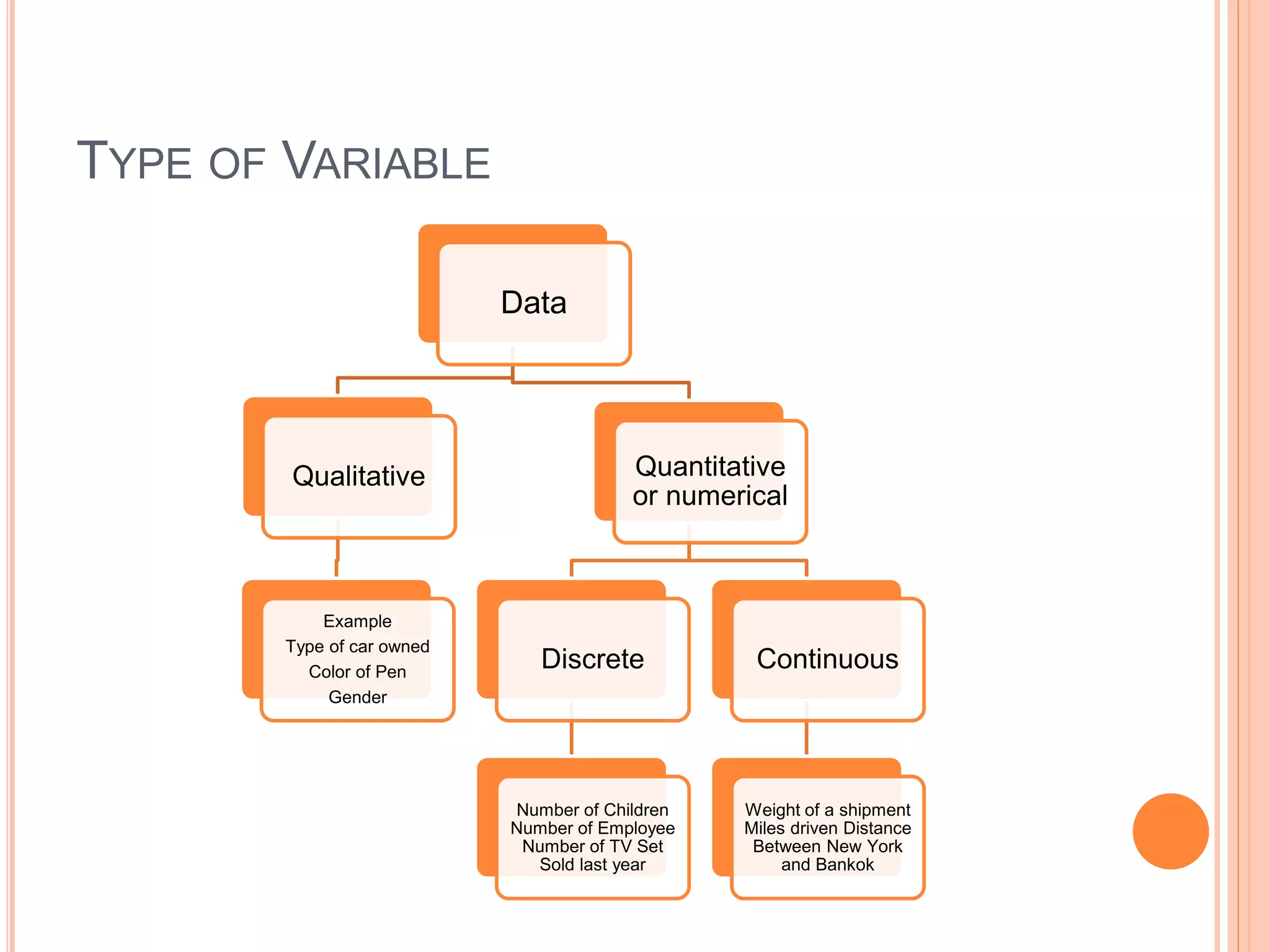
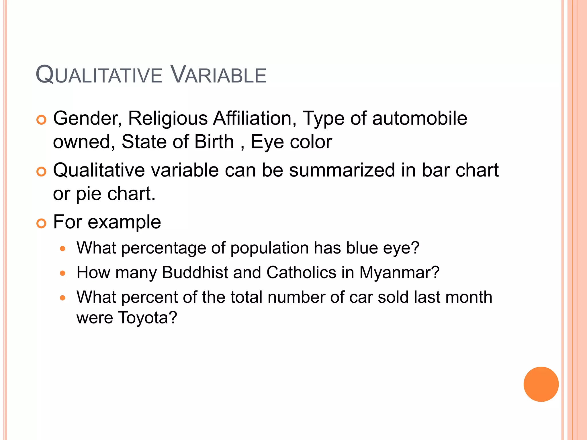
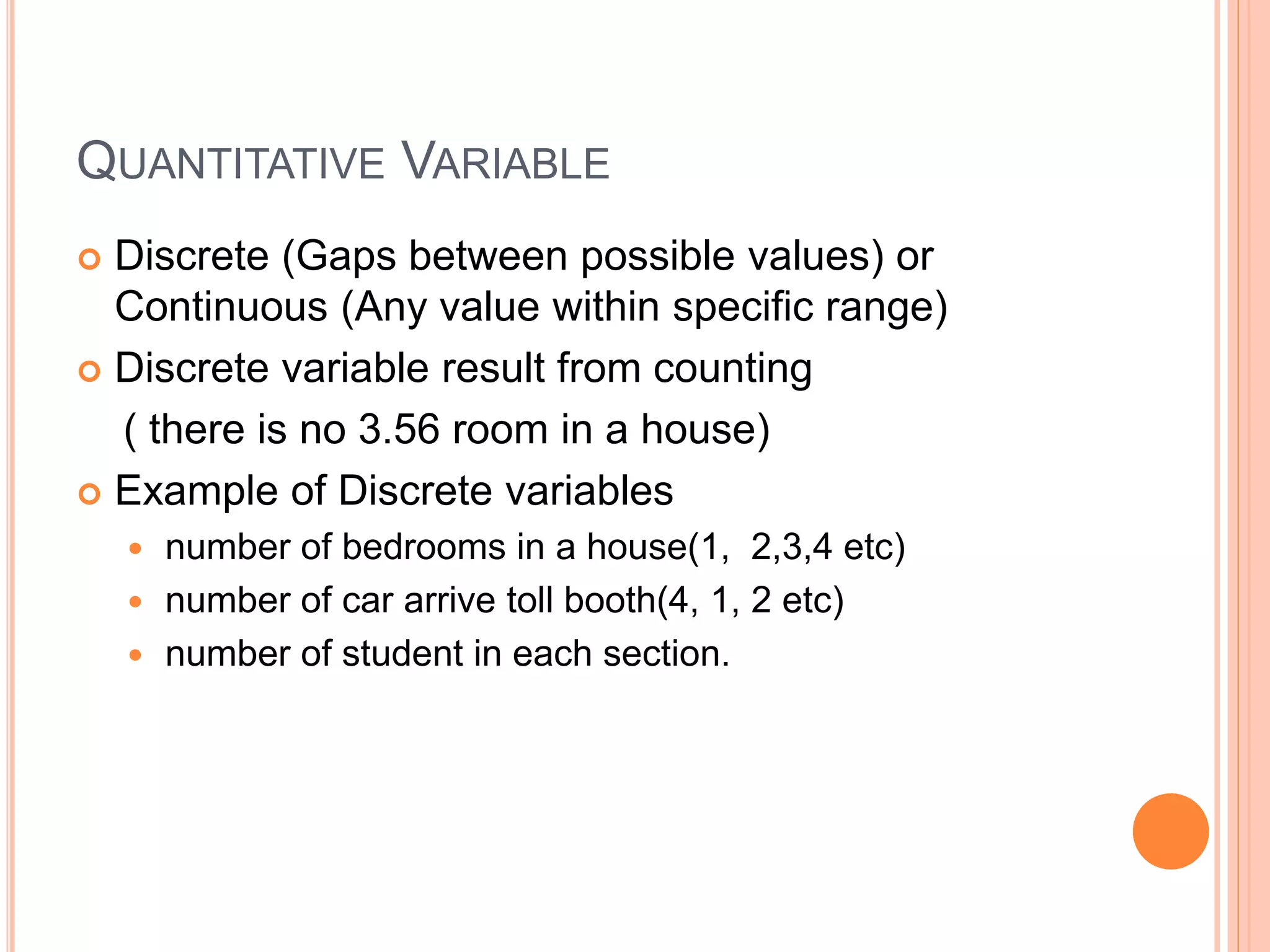
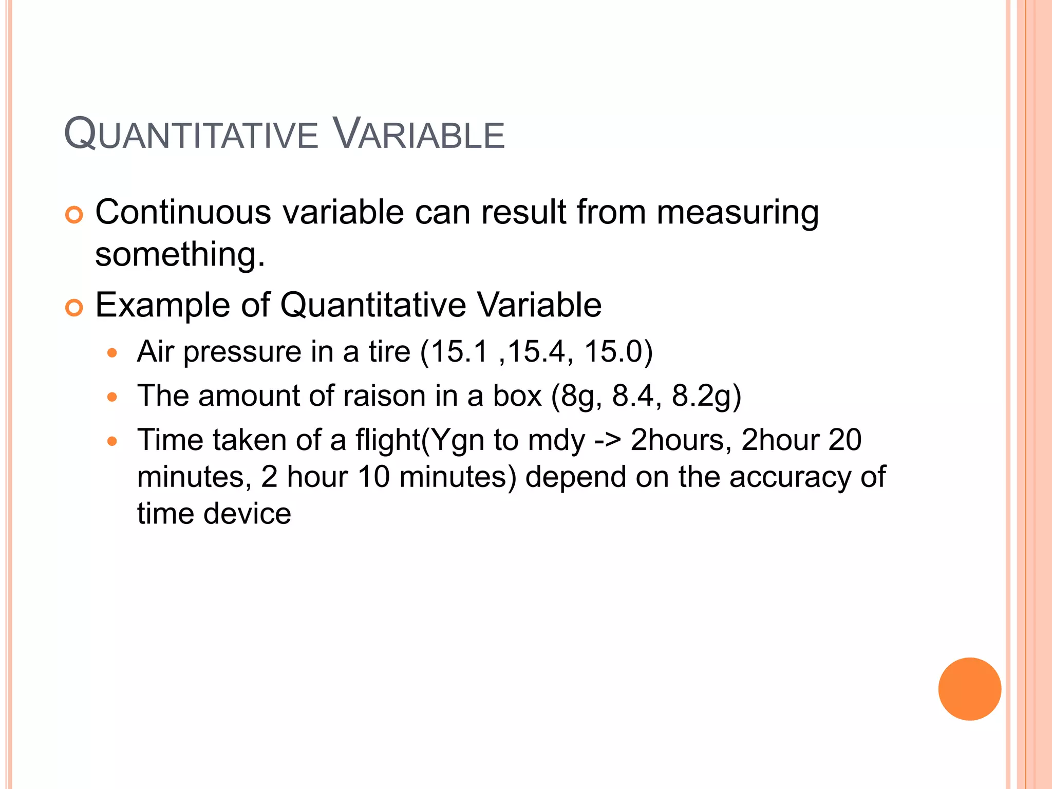
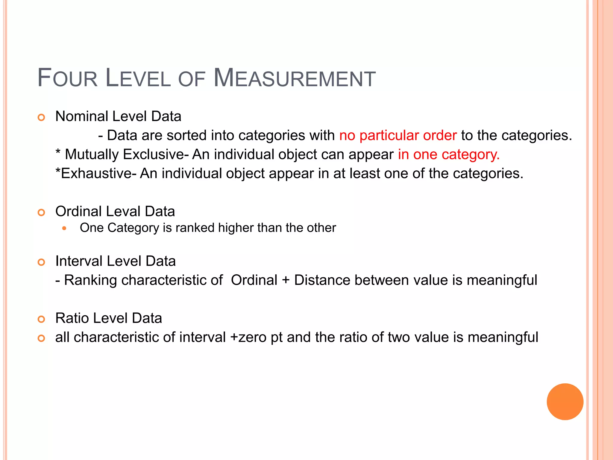
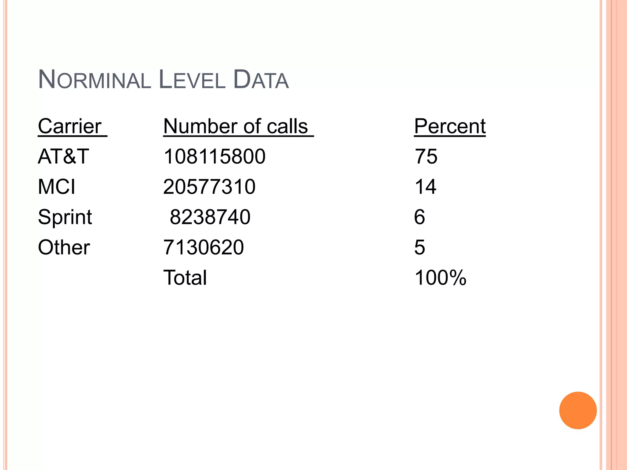
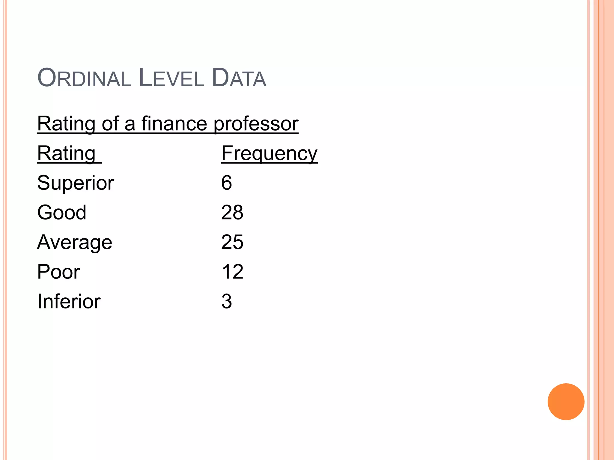
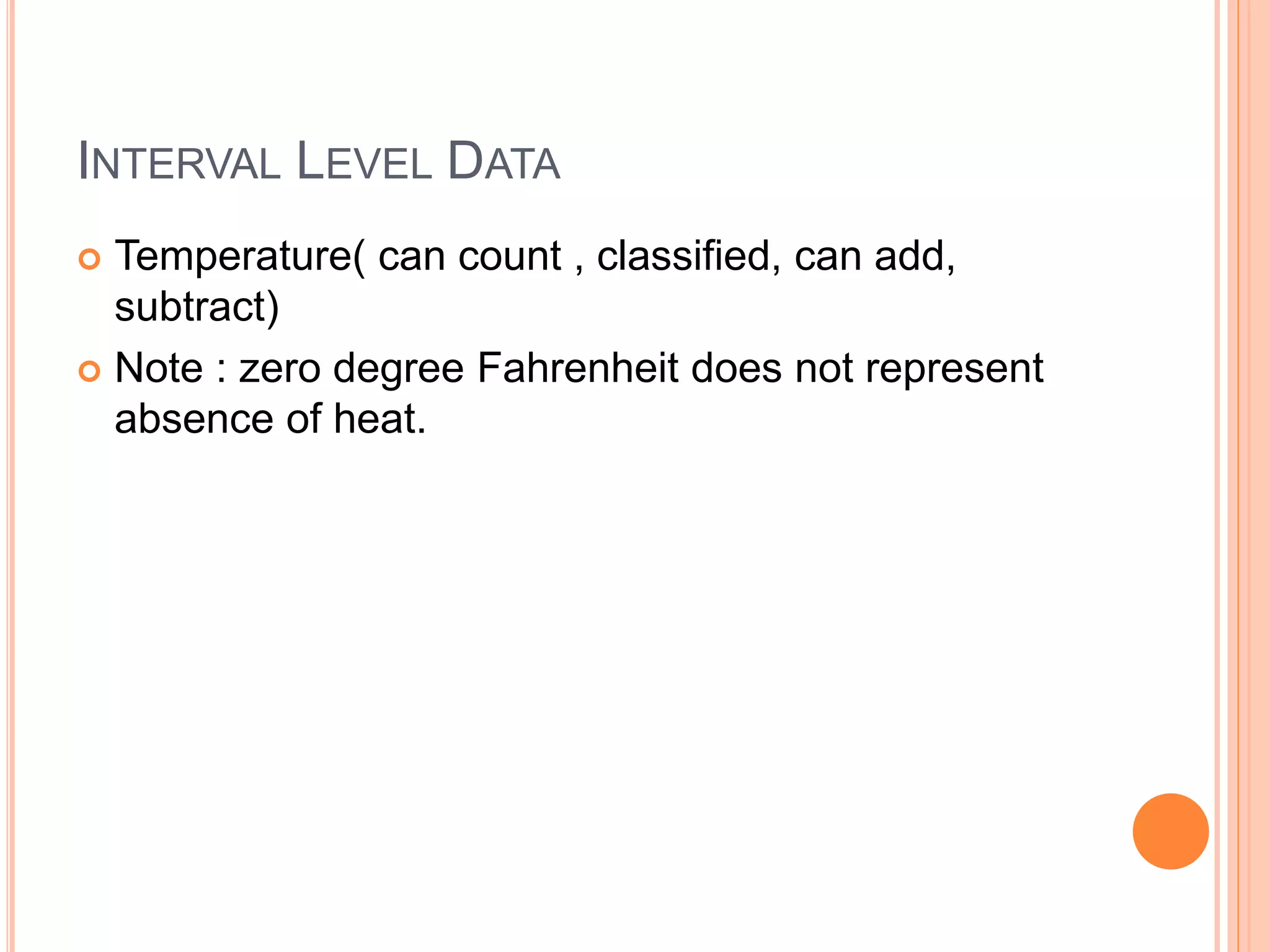
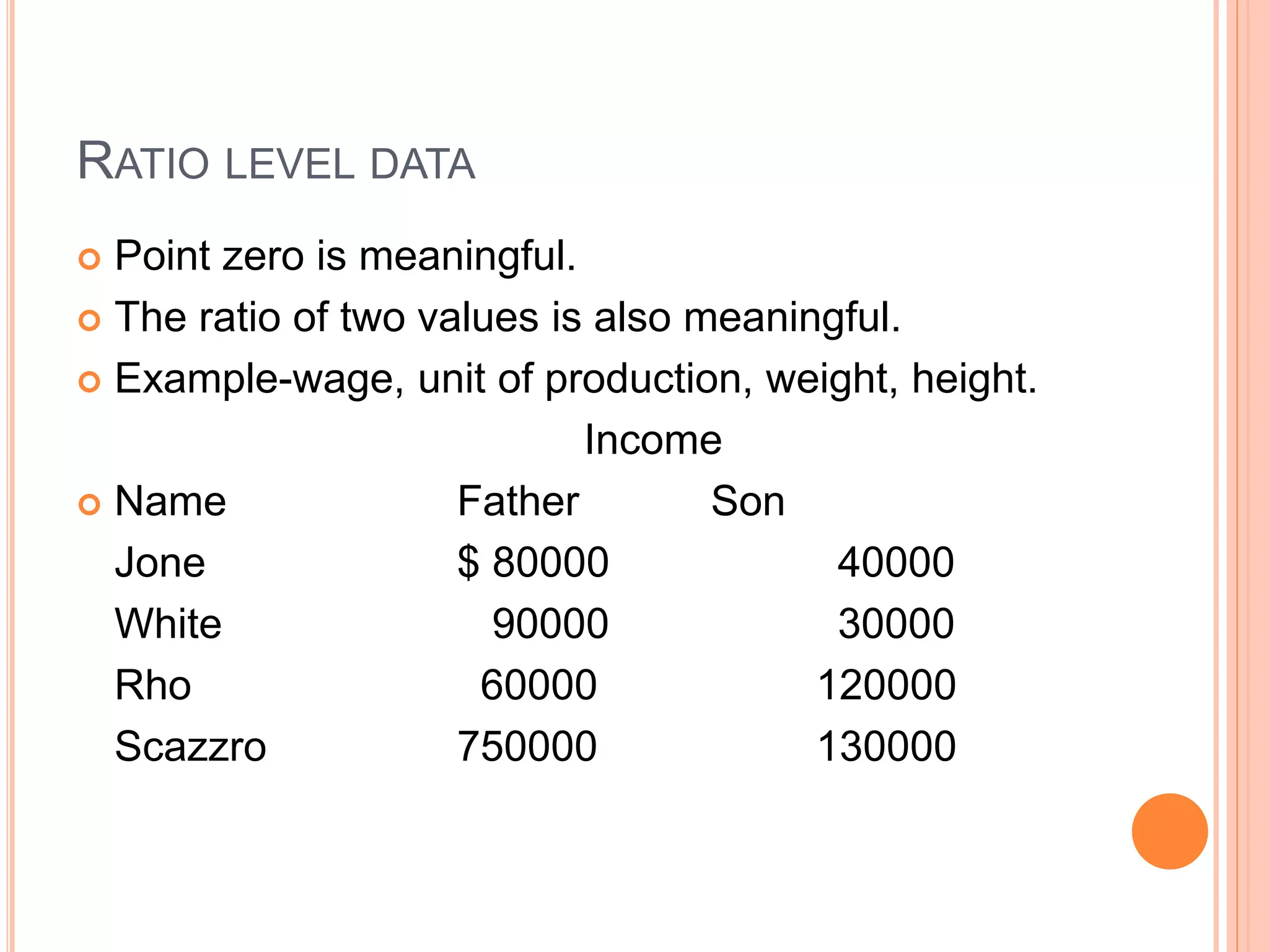
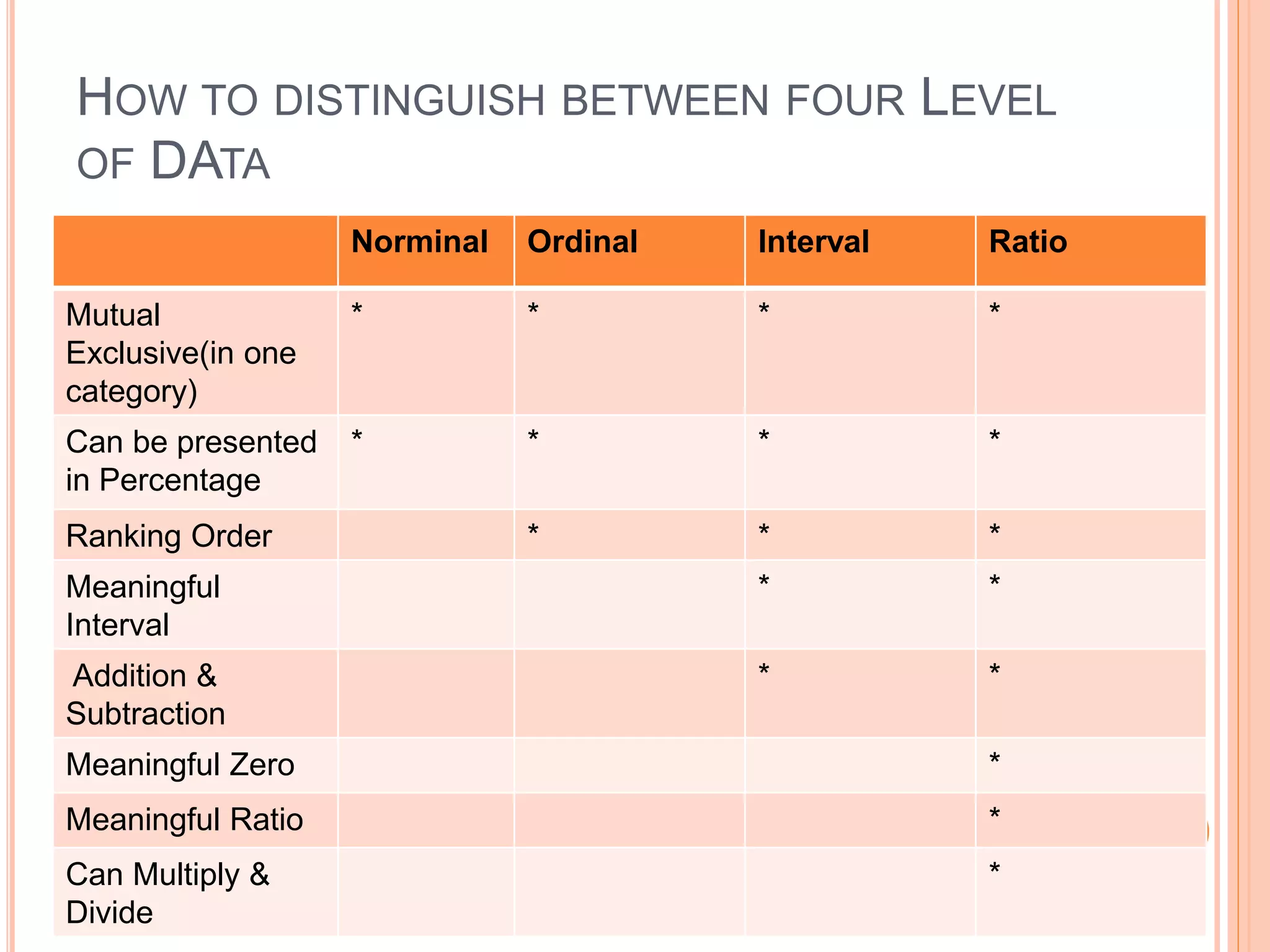
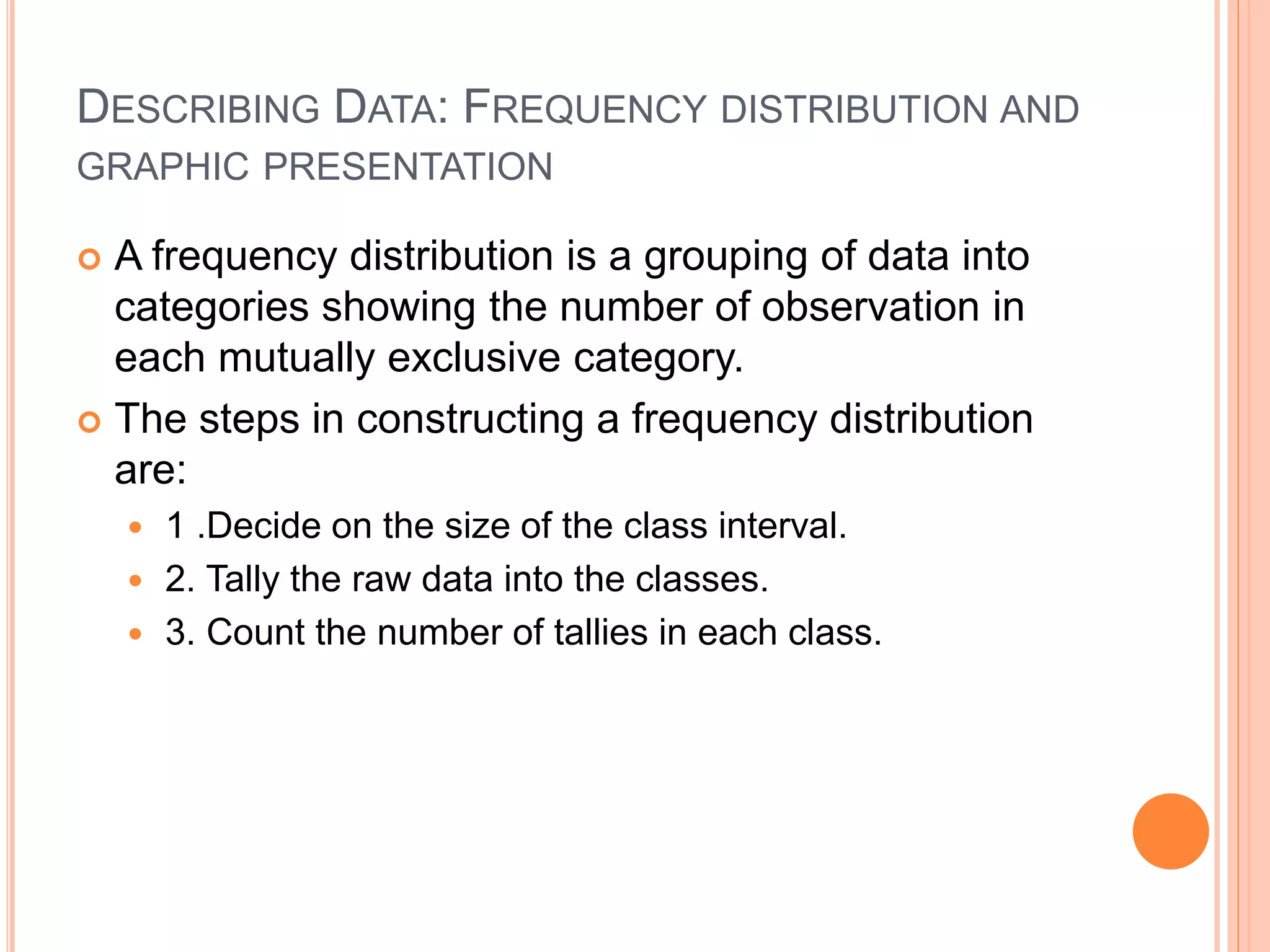
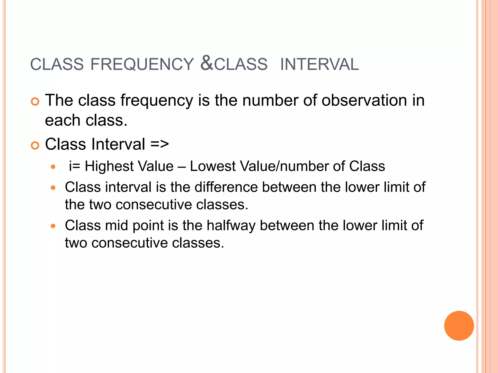
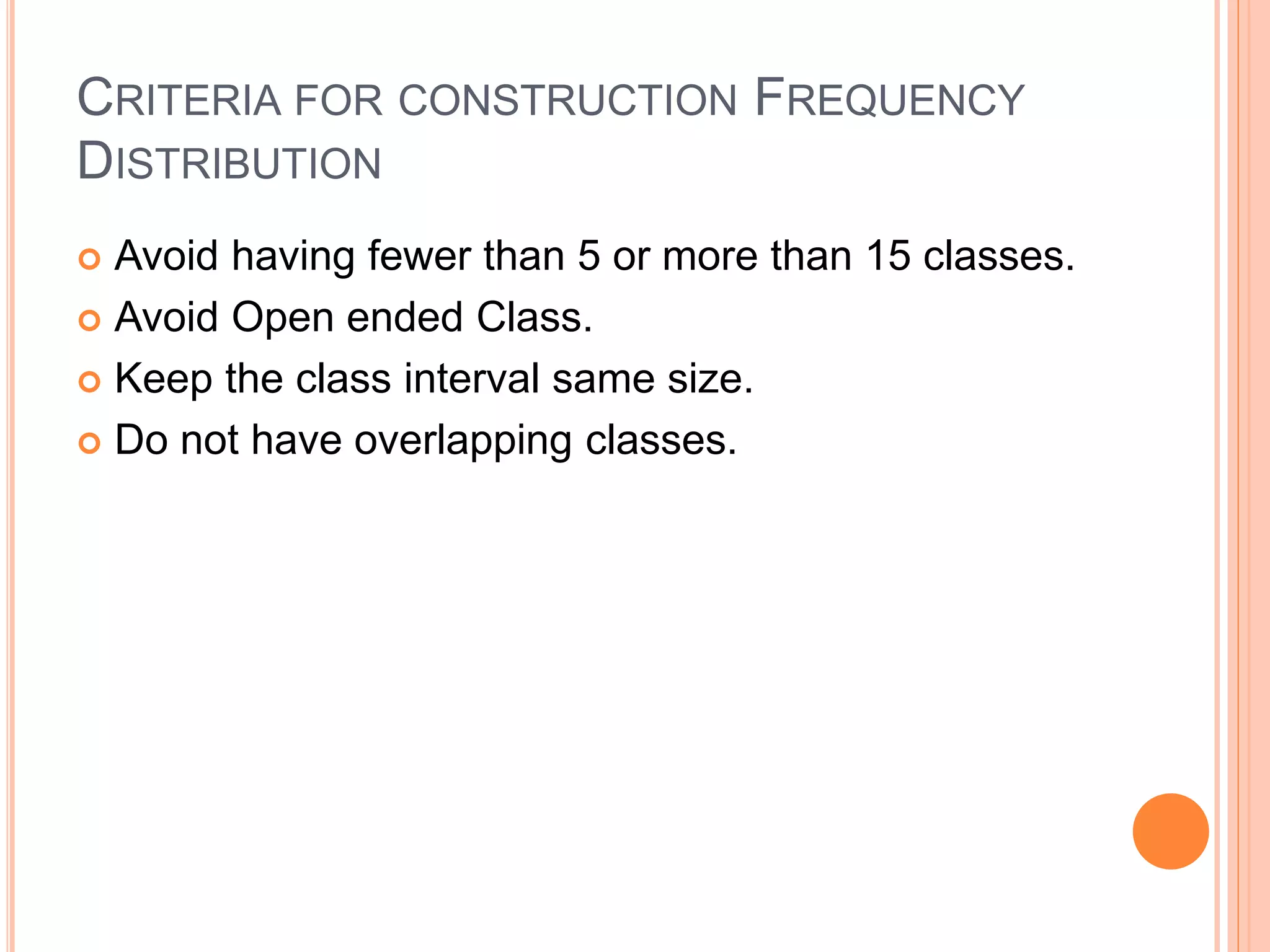
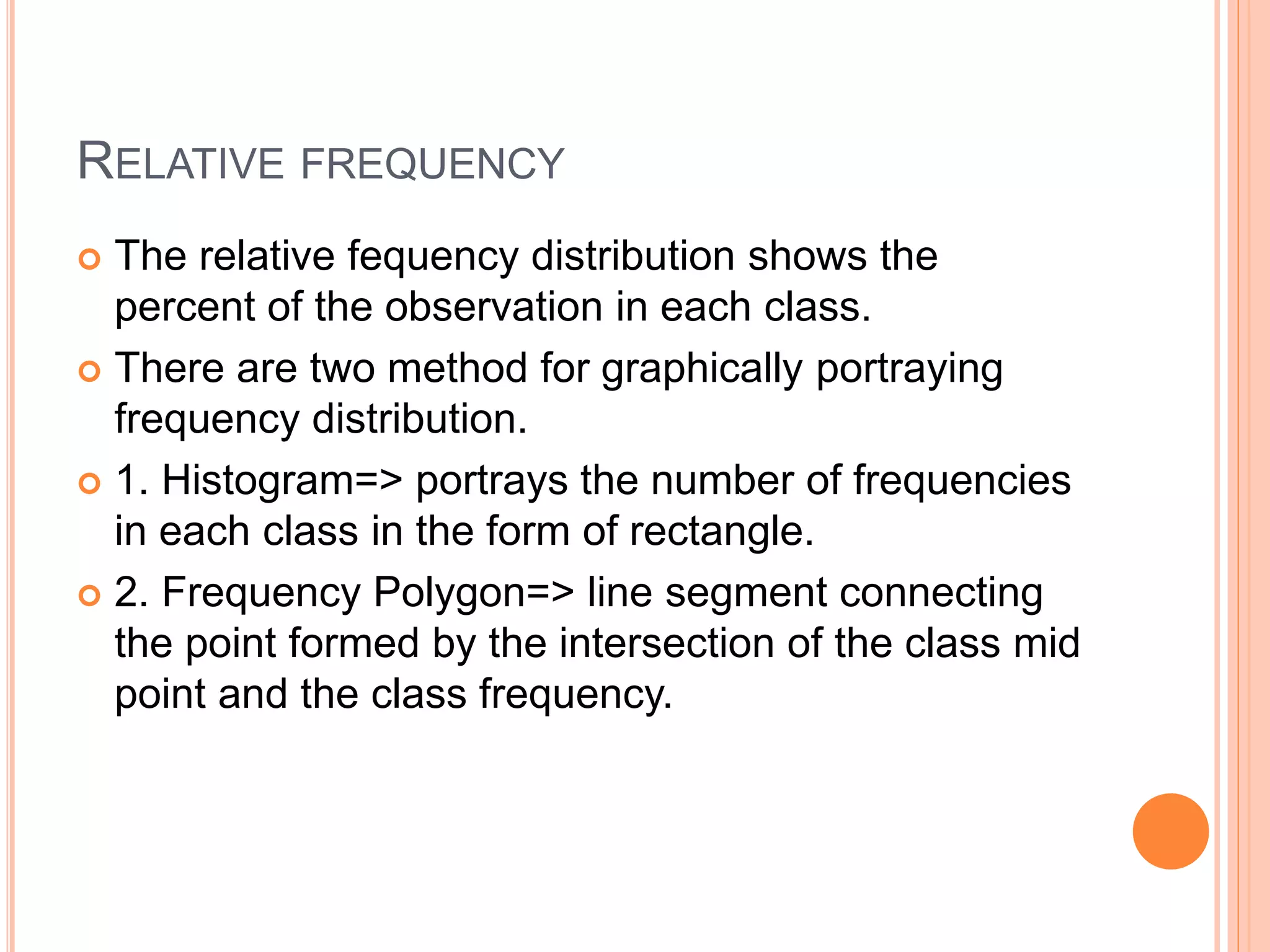
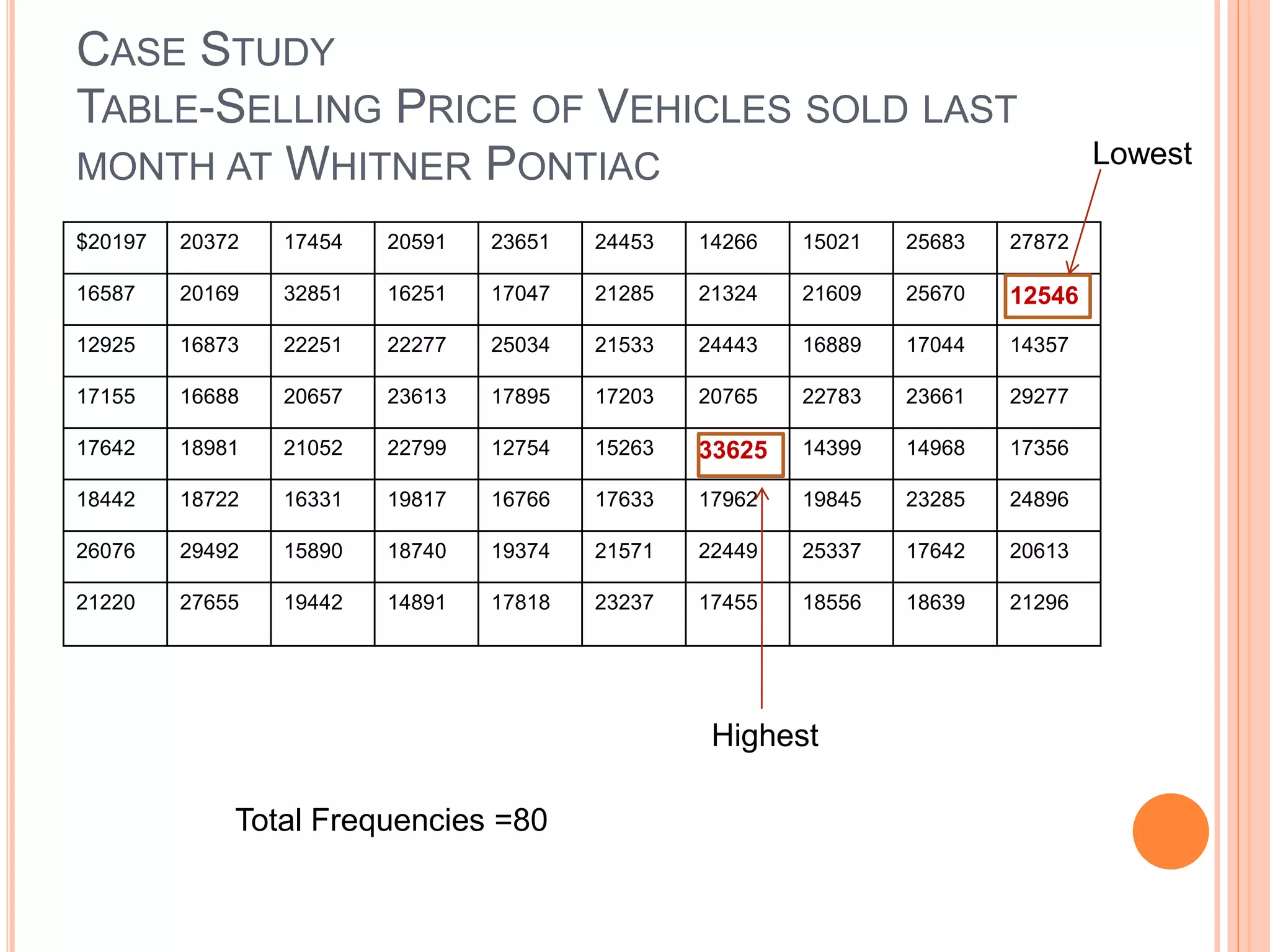
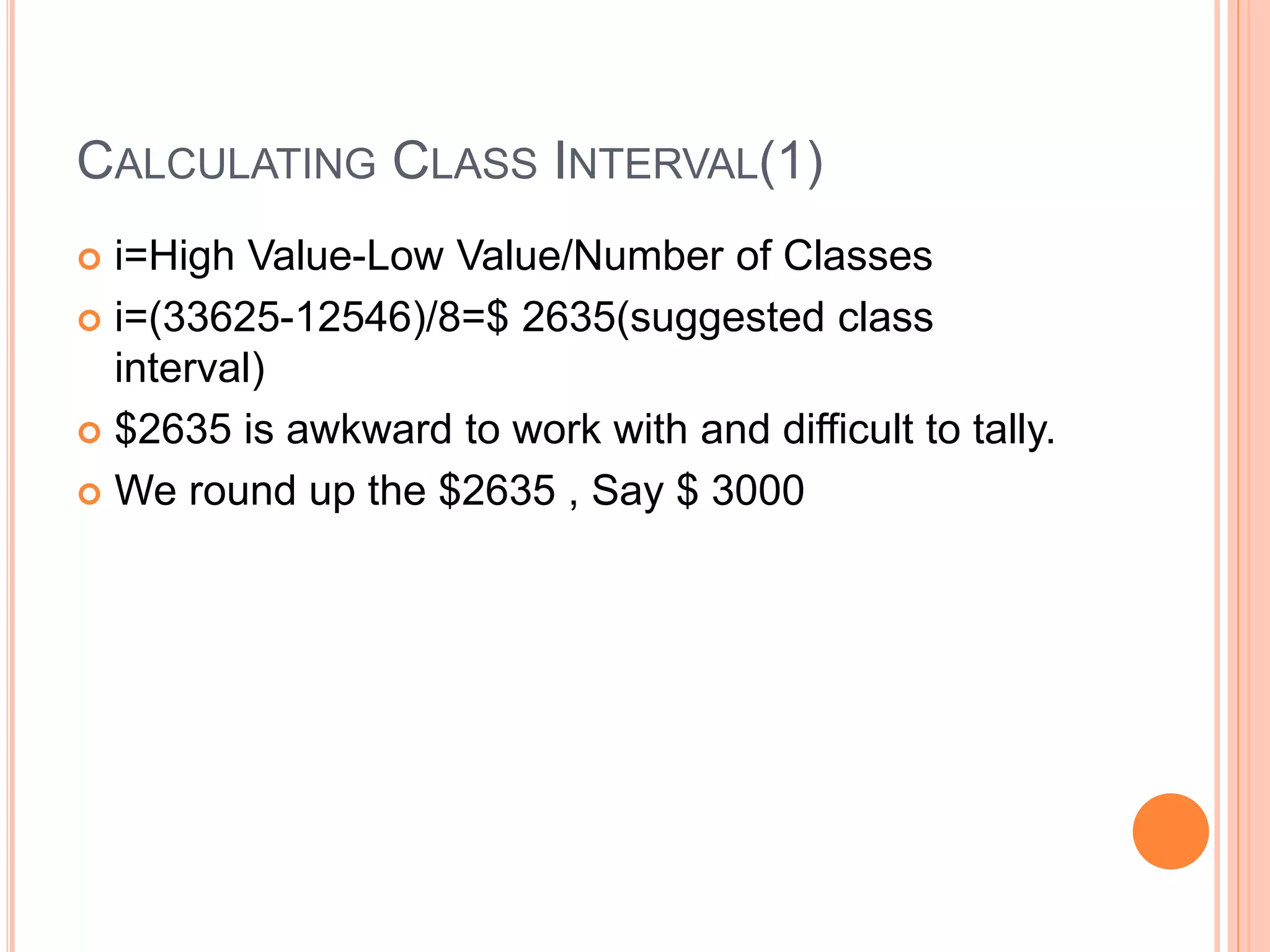
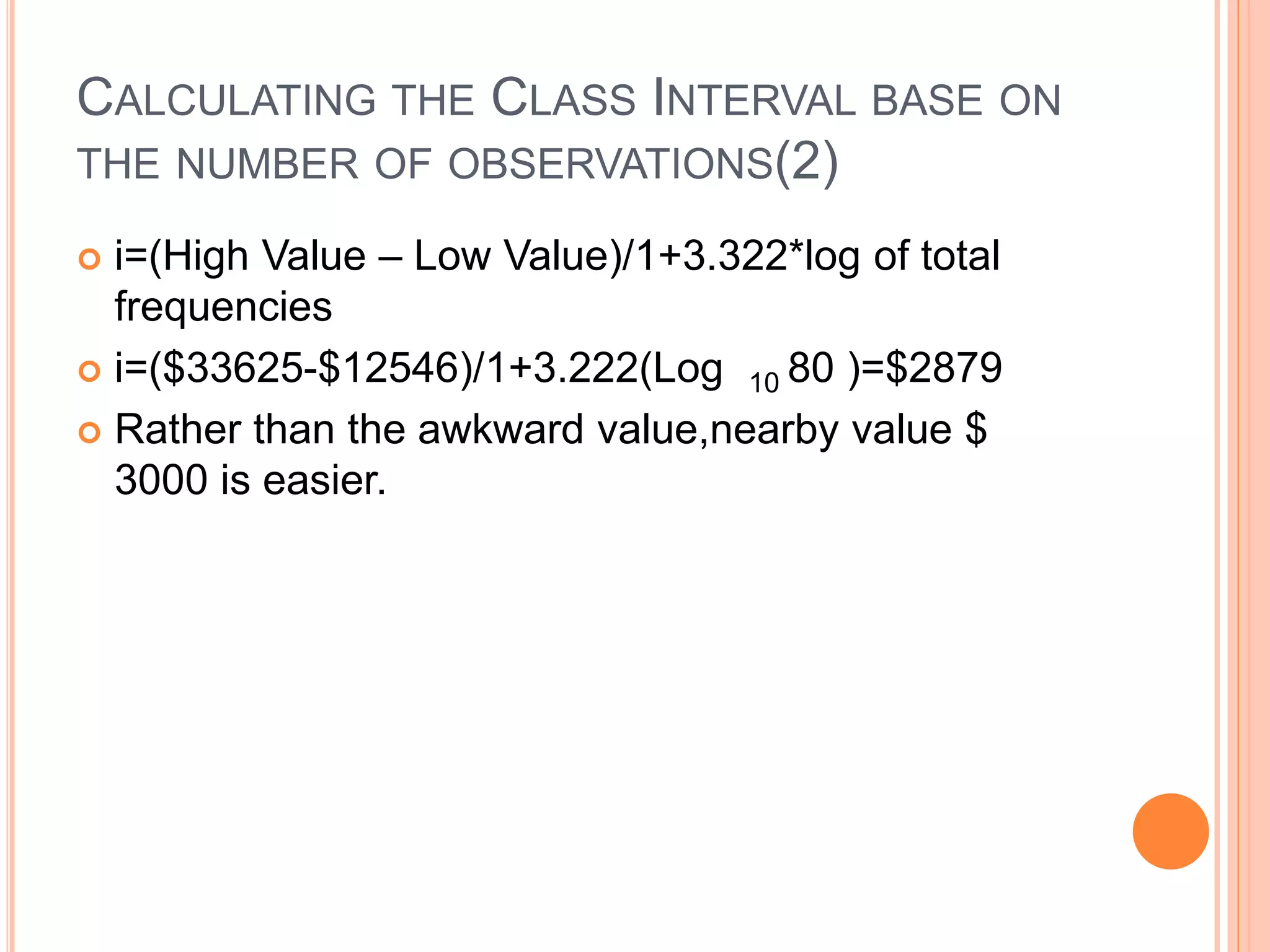
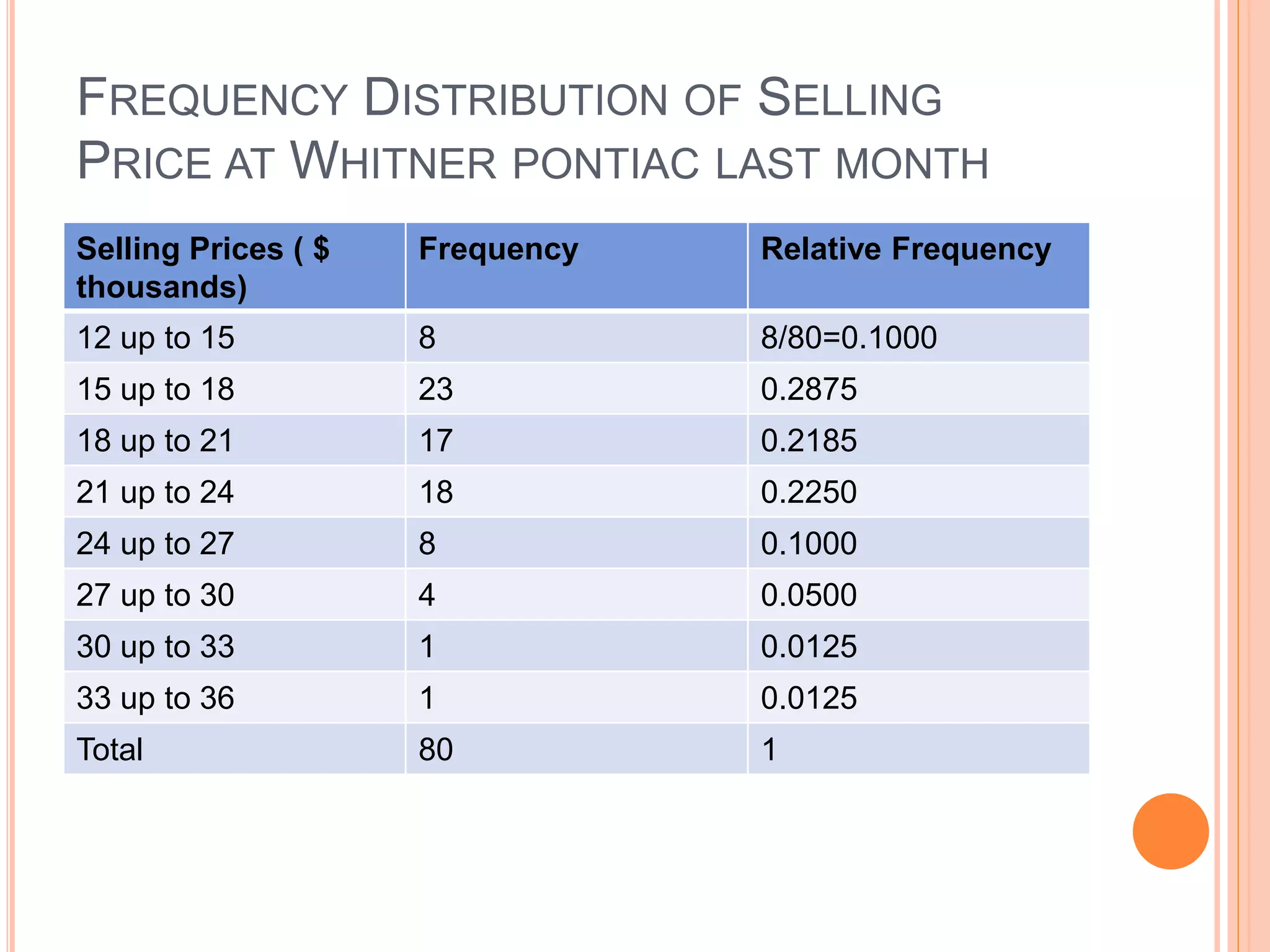
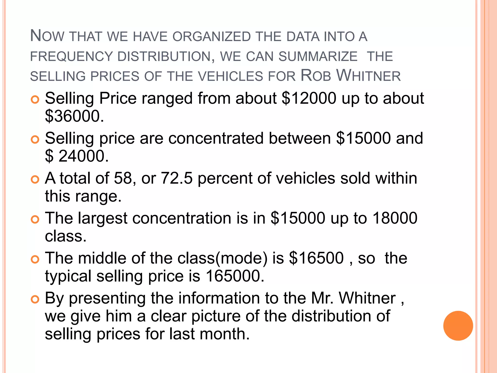
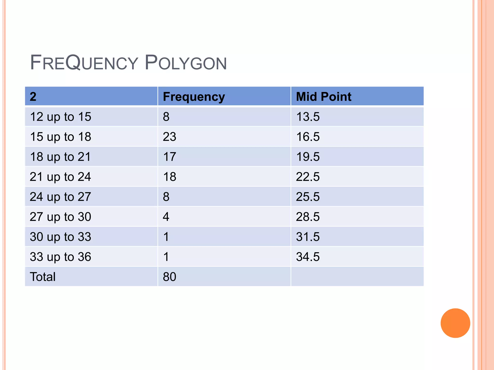
TYPES OF DATA 
Presented by Hnin Thiri Chaw (9PhD-3)
OUTLINE 
 What is Statistics ? 
 Type of Statistics 
 Type of Sampling 
 Four Level of Measurement 
 Describing Data: Frequency Distributions and 
Graphic Presentation
WHAT IS STATISTICS? 
 The science of collecting, organizing, presenting, 
analyzing and interpreting data to assist in making 
more effective decision.
TO MAKE IMPORTANT DECISION 
 Determine existing information and additional 
information. 
 Gather additional information, but does not lead 
misleading result. 
 Summarize information in a useful and informative 
manner. 
 Analyze the available information. 
 Draw conclusion while assessing the risk and 
incorrect conclusion
TYPE OF STATISTICS 
 Descriptive Statistics(Without analysis) 
 Method of organizing, summarizing and presenting data 
in an informative way. 
 Inferential Statistics(With analysis) 
 Population(A collection of all possible individuals, 
objects, or measurements of interest.) 
 Sample (A portion, or part of the population of interest)
SAMPLING A POPULATION 
 Reason 
 Impossible to check or locate all the members of the 
population 
 Cost of Studying all the items in the population may be 
prohabitive. 
 The result of a sample is the estimate of the population 
parameter thus saving time and money. 
 It may be too time consuming to contact all the 
members of the population.
TYPE OF SAMPLE 
Type of 
Sample 
Probability 
Sample 
Simple 
Random 
Sampling 
Systematic 
Sampling 
Stratified 
Sampling 
Cluster 
Sampling 
Non Probability 
Sample 
Panel 
Sampling 
Convenience 
Sampling
PROBABILITY SAMPLE 
 Simple Random Sample 
 all members of the population has the same chance of 
being selected for a sample. 
 Systematic Sample 
 A random starting point is selected, then every k item is 
selected for the sample. 
 Stratified Sample 
 Population is divided into several groups or strata and 
then a sample is selected from each stratum. 
 Cluster Sample 
 Primary units and then samples are drawn from the 
primary unit.
NONPROBABILITY SAMPLING 
 Inclusion in the sample is based on the judgment of 
the person conducting the sample. 
 Non Probability samples may lead to biased result.
SAMPLING ERROR 
 The difference between the population parameter 
and the sample statistic are called the sampling 
error.
TYPE OF VARIABLE 
Data 
Qualitative 
Example 
Type of car owned 
Color of Pen 
Gender 
Quantitative 
or numerical 
Discrete 
Number of Children 
Number of Employee 
Number of TV Set 
Sold last year 
Continuous 
Weight of a shipment 
Miles driven Distance 
Between New York 
and Bankok
QUALITATIVE VARIABLE 
 Gender, Religious Affiliation, Type of automobile 
owned, State of Birth , Eye color 
 Qualitative variable can be summarized in bar chart 
or pie chart. 
 For example 
 What percentage of population has blue eye? 
 How many Buddhist and Catholics in Myanmar? 
 What percent of the total number of car sold last month 
were Toyota?
QUANTITATIVE VARIABLE 
 Discrete (Gaps between possible values) or 
Continuous (Any value within specific range) 
 Discrete variable result from counting 
( there is no 3.56 room in a house) 
 Example of Discrete variables 
 number of bedrooms in a house(1, 2,3,4 etc) 
 number of car arrive toll booth(4, 1, 2 etc) 
 number of student in each section.
QUANTITATIVE VARIABLE 
 Continuous variable can result from measuring 
something. 
 Example of Quantitative Variable 
 Air pressure in a tire (15.1 ,15.4, 15.0) 
 The amount of raison in a box (8g, 8.4, 8.2g) 
 Time taken of a flight(Ygn to mdy -> 2hours, 2hour 20 
minutes, 2 hour 10 minutes) depend on the accuracy of 
time device
SOURCE OF STATISTICAL DATA 
 Secondary Data ( Government publication, 
Statistical year book, Published Data)
FOUR LEVEL OF MEASUREMENT 
 Nominal Level Data 
- Data are sorted into categories with no particular order to the categories. 
* Mutually Exclusive- An individual object can appear in one category. 
*Exhaustive- An individual object appear in at least one of the categories. 
 Ordinal Leval Data 
 One Category is ranked higher than the other 
 Interval Level Data 
- Ranking characteristic of Ordinal + Distance between value is meaningful 
 Ratio Level Data 
 all characteristic of interval +zero pt and the ratio of two value is meaningful
NORMINAL LEVEL DATA 
Carrier Number of calls Percent 
AT&T 108115800 75 
MCI 20577310 14 
Sprint 8238740 6 
Other 7130620 5 
Total 100%
ORDINAL LEVEL DATA 
Rating of a finance professor 
Rating Frequency 
Superior 6 
Good 28 
Average 25 
Poor 12 
Inferior 3
INTERVAL LEVEL DATA 
 Temperature( can count , classified, can add, 
subtract) 
 Note : zero degree Fahrenheit does not represent 
absence of heat.
RATIO LEVEL DATA 
 Point zero is meaningful. 
 The ratio of two values is also meaningful. 
 Example-wage, unit of production, weight, height. 
Income 
 Name Father Son 
Jone $ 80000 40000 
White 90000 30000 
Rho 60000 120000 
Scazzro 750000 130000
HOW TO DISTINGUISH BETWEEN FOUR LEVEL 
OF DATA 
Norminal Ordinal Interval Ratio 
Mutual 
Exclusive(in one 
category) 
* * * * 
Can be presented 
in Percentage 
* * * * 
Ranking Order * * * 
Meaningful 
* * 
Interval 
Addition & 
Subtraction 
* * 
Meaningful Zero * 
Meaningful Ratio * 
Can Multiply & 
* 
Divide
WHAT IS THE LEVEL OF MEASUREMENT FOR 
EACH OF THE VARIABLE? 
 Student Grade point Average 
?
Ans: Interval
WHAT IS THE LEVEL OF MEASUREMENT FOR 
EACH OF THE VARIABLE? 
Ranking of Student by freshmen, junior , senior 
?
Ans: Ordinal
WHAT IS THE LEVEL OF MEASUREMENT FOR 
EACH OF THE VARIABLE? 
Number of hours Student Study per week 
?
Ans: Ratio
DESCRIBING DATA: FREQUENCY DISTRIBUTION AND 
GRAPHIC PRESENTATION 
 A frequency distribution is a grouping of data into 
categories showing the number of observation in 
each mutually exclusive category. 
 The steps in constructing a frequency distribution 
are: 
 1 .Decide on the size of the class interval. 
 2. Tally the raw data into the classes. 
 3. Count the number of tallies in each class.
CLASS FREQUENCY &CLASS INTERVAL 
 The class frequency is the number of observation in 
each class. 
 Class Interval => 
 i= Highest Value – Lowest Value/number of Class 
 Class interval is the difference between the lower limit of 
the two consecutive classes. 
 Class mid point is the halfway between the lower limit of 
two consecutive classes.
CRITERIA FOR CONSTRUCTION FREQUENCY 
DISTRIBUTION 
 Avoid having fewer than 5 or more than 15 classes. 
 Avoid Open ended Class. 
 Keep the class interval same size. 
 Do not have overlapping classes.
RELATIVE FREQUENCY 
 The relative fequency distribution shows the 
percent of the observation in each class. 
 There are two method for graphically portraying 
frequency distribution. 
 1. Histogram=> portrays the number of frequencies 
in each class in the form of rectangle. 
 2. Frequency Polygon=> line segment connecting 
the point formed by the intersection of the class mid 
point and the class frequency.
ANOTHER ALTERNATIVE 
 Line Chart => ideal for showing the trend of sale, 
income over time. 
 Bar Chart => showing the changes in business and 
economic data over time. 
 Pie Chart => the percent of various components are 
of total.
CASE STUDY 
TABLE-SELLING PRICE OF VEHICLES SOLD LAST 
MONTH AT WHITNER PONTIAC 
$20197 20372 17454 20591 23651 24453 14266 15021 25683 27872 
16587 20169 32851 16251 17047 21285 21324 21609 25670 12546 
12925 16873 22251 22277 25034 21533 24443 16889 17044 14357 
17155 16688 20657 23613 17895 17203 20765 22783 23661 29277 
17642 18981 21052 22799 12754 15263 33625 14399 14968 17356 
18442 18722 16331 19817 16766 17633 17962 19845 23285 24896 
26076 29492 15890 18740 19374 21571 22449 25337 17642 20613 
21220 27655 19442 14891 17818 23237 17455 18556 18639 21296 
Lowest 
Highest 
Total Frequencies =80
CALCULATING CLASS INTERVAL(1) 
 i=High Value-Low Value/Number of Classes 
 i=(33625-12546)/8=$ 2635(suggested class 
interval) 
 $2635 is awkward to work with and difficult to tally. 
 We round up the $2635 , Say $ 3000
CALCULATING THE CLASS INTERVAL BASE ON 
THE NUMBER OF OBSERVATIONS(2) 
 i=(High Value – Low Value)/1+3.322*log of total 
frequencies 
 i=($33625-$12546)/1+3.222(Log 10 80 )=$2879 
 Rather than the awkward value,nearby value $ 
3000 is easier.
FREQUENCY DISTRIBUTION OF SELLING 
PRICE AT WHITNER PONTIAC LAST MONTH 
Selling Prices ( $ 
thousands) 
Frequency Relative Frequency 
12 up to 15 8 8/80=0.1000 
15 up to 18 23 0.2875 
18 up to 21 17 0.2185 
21 up to 24 18 0.2250 
24 up to 27 8 0.1000 
27 up to 30 4 0.0500 
30 up to 33 1 0.0125 
33 up to 36 1 0.0125 
Total 80 1
NOW THAT WE HAVE ORGANIZED THE DATA INTO A 
FREQUENCY DISTRIBUTION, WE CAN SUMMARIZE THE 
SELLING PRICES OF THE VEHICLES FOR ROB WHITNER 
 Selling Price ranged from about $12000 up to about 
$36000. 
 Selling price are concentrated between $15000 and 
$ 24000. 
 A total of 58, or 72.5 percent of vehicles sold within 
this range. 
 The largest concentration is in $15000 up to 18000 
class. 
 The middle of the class(mode) is $16500 , so the 
typical selling price is 165000. 
 By presenting the information to the Mr. Whitner , 
we give him a clear picture of the distribution of 
selling prices for last month.
FREQUENCY POLYGON 
2 Frequency Mid Point 
12 up to 15 8 13.5 
15 up to 18 23 16.5 
18 up to 21 17 19.5 
21 up to 24 18 22.5 
24 up to 27 8 25.5 
27 up to 30 4 28.5 
30 up to 33 1 31.5 
33 up to 36 1 34.5 
Total 80
 Reference 
 Statistical Techniques in business and economics 
 Author : Robert D. Mason 
Douglas A. Lind 
William G. Marchal
“SHARING IS CARING” 
THANKS FOR YOUR ATTENTION!

Type of data @ web mining discussion

  • 1.
    TYPES OF DATA Presented by Hnin Thiri Chaw (9PhD-3)
  • 2.
    OUTLINE  Whatis Statistics ?  Type of Statistics  Type of Sampling  Four Level of Measurement  Describing Data: Frequency Distributions and Graphic Presentation
  • 3.
    WHAT IS STATISTICS?  The science of collecting, organizing, presenting, analyzing and interpreting data to assist in making more effective decision.
  • 4.
    TO MAKE IMPORTANTDECISION  Determine existing information and additional information.  Gather additional information, but does not lead misleading result.  Summarize information in a useful and informative manner.  Analyze the available information.  Draw conclusion while assessing the risk and incorrect conclusion
  • 5.
    TYPE OF STATISTICS  Descriptive Statistics(Without analysis)  Method of organizing, summarizing and presenting data in an informative way.  Inferential Statistics(With analysis)  Population(A collection of all possible individuals, objects, or measurements of interest.)  Sample (A portion, or part of the population of interest)
  • 6.
    SAMPLING A POPULATION  Reason  Impossible to check or locate all the members of the population  Cost of Studying all the items in the population may be prohabitive.  The result of a sample is the estimate of the population parameter thus saving time and money.  It may be too time consuming to contact all the members of the population.
  • 7.
    TYPE OF SAMPLE Type of Sample Probability Sample Simple Random Sampling Systematic Sampling Stratified Sampling Cluster Sampling Non Probability Sample Panel Sampling Convenience Sampling
  • 8.
    PROBABILITY SAMPLE Simple Random Sample  all members of the population has the same chance of being selected for a sample.  Systematic Sample  A random starting point is selected, then every k item is selected for the sample.  Stratified Sample  Population is divided into several groups or strata and then a sample is selected from each stratum.  Cluster Sample  Primary units and then samples are drawn from the primary unit.
  • 9.
    NONPROBABILITY SAMPLING Inclusion in the sample is based on the judgment of the person conducting the sample.  Non Probability samples may lead to biased result.
  • 10.
    SAMPLING ERROR The difference between the population parameter and the sample statistic are called the sampling error.
  • 11.
    TYPE OF VARIABLE Data Qualitative Example Type of car owned Color of Pen Gender Quantitative or numerical Discrete Number of Children Number of Employee Number of TV Set Sold last year Continuous Weight of a shipment Miles driven Distance Between New York and Bankok
  • 12.
    QUALITATIVE VARIABLE Gender, Religious Affiliation, Type of automobile owned, State of Birth , Eye color  Qualitative variable can be summarized in bar chart or pie chart.  For example  What percentage of population has blue eye?  How many Buddhist and Catholics in Myanmar?  What percent of the total number of car sold last month were Toyota?
  • 13.
    QUANTITATIVE VARIABLE Discrete (Gaps between possible values) or Continuous (Any value within specific range)  Discrete variable result from counting ( there is no 3.56 room in a house)  Example of Discrete variables  number of bedrooms in a house(1, 2,3,4 etc)  number of car arrive toll booth(4, 1, 2 etc)  number of student in each section.
  • 14.
    QUANTITATIVE VARIABLE Continuous variable can result from measuring something.  Example of Quantitative Variable  Air pressure in a tire (15.1 ,15.4, 15.0)  The amount of raison in a box (8g, 8.4, 8.2g)  Time taken of a flight(Ygn to mdy -> 2hours, 2hour 20 minutes, 2 hour 10 minutes) depend on the accuracy of time device
  • 15.
    SOURCE OF STATISTICALDATA  Secondary Data ( Government publication, Statistical year book, Published Data)
  • 16.
    FOUR LEVEL OFMEASUREMENT  Nominal Level Data - Data are sorted into categories with no particular order to the categories. * Mutually Exclusive- An individual object can appear in one category. *Exhaustive- An individual object appear in at least one of the categories.  Ordinal Leval Data  One Category is ranked higher than the other  Interval Level Data - Ranking characteristic of Ordinal + Distance between value is meaningful  Ratio Level Data  all characteristic of interval +zero pt and the ratio of two value is meaningful
  • 17.
    NORMINAL LEVEL DATA Carrier Number of calls Percent AT&T 108115800 75 MCI 20577310 14 Sprint 8238740 6 Other 7130620 5 Total 100%
  • 18.
    ORDINAL LEVEL DATA Rating of a finance professor Rating Frequency Superior 6 Good 28 Average 25 Poor 12 Inferior 3
  • 19.
    INTERVAL LEVEL DATA  Temperature( can count , classified, can add, subtract)  Note : zero degree Fahrenheit does not represent absence of heat.
  • 20.
    RATIO LEVEL DATA  Point zero is meaningful.  The ratio of two values is also meaningful.  Example-wage, unit of production, weight, height. Income  Name Father Son Jone $ 80000 40000 White 90000 30000 Rho 60000 120000 Scazzro 750000 130000
  • 21.
    HOW TO DISTINGUISHBETWEEN FOUR LEVEL OF DATA Norminal Ordinal Interval Ratio Mutual Exclusive(in one category) * * * * Can be presented in Percentage * * * * Ranking Order * * * Meaningful * * Interval Addition & Subtraction * * Meaningful Zero * Meaningful Ratio * Can Multiply & * Divide
  • 22.
    WHAT IS THELEVEL OF MEASUREMENT FOR EACH OF THE VARIABLE?  Student Grade point Average ?
  • 23.
  • 24.
    WHAT IS THELEVEL OF MEASUREMENT FOR EACH OF THE VARIABLE? Ranking of Student by freshmen, junior , senior ?
  • 25.
  • 26.
    WHAT IS THELEVEL OF MEASUREMENT FOR EACH OF THE VARIABLE? Number of hours Student Study per week ?
  • 27.
  • 28.
    DESCRIBING DATA: FREQUENCYDISTRIBUTION AND GRAPHIC PRESENTATION  A frequency distribution is a grouping of data into categories showing the number of observation in each mutually exclusive category.  The steps in constructing a frequency distribution are:  1 .Decide on the size of the class interval.  2. Tally the raw data into the classes.  3. Count the number of tallies in each class.
  • 29.
    CLASS FREQUENCY &CLASSINTERVAL  The class frequency is the number of observation in each class.  Class Interval =>  i= Highest Value – Lowest Value/number of Class  Class interval is the difference between the lower limit of the two consecutive classes.  Class mid point is the halfway between the lower limit of two consecutive classes.
  • 30.
    CRITERIA FOR CONSTRUCTIONFREQUENCY DISTRIBUTION  Avoid having fewer than 5 or more than 15 classes.  Avoid Open ended Class.  Keep the class interval same size.  Do not have overlapping classes.
  • 31.
    RELATIVE FREQUENCY The relative fequency distribution shows the percent of the observation in each class.  There are two method for graphically portraying frequency distribution.  1. Histogram=> portrays the number of frequencies in each class in the form of rectangle.  2. Frequency Polygon=> line segment connecting the point formed by the intersection of the class mid point and the class frequency.
  • 32.
    ANOTHER ALTERNATIVE Line Chart => ideal for showing the trend of sale, income over time.  Bar Chart => showing the changes in business and economic data over time.  Pie Chart => the percent of various components are of total.
  • 33.
    CASE STUDY TABLE-SELLINGPRICE OF VEHICLES SOLD LAST MONTH AT WHITNER PONTIAC $20197 20372 17454 20591 23651 24453 14266 15021 25683 27872 16587 20169 32851 16251 17047 21285 21324 21609 25670 12546 12925 16873 22251 22277 25034 21533 24443 16889 17044 14357 17155 16688 20657 23613 17895 17203 20765 22783 23661 29277 17642 18981 21052 22799 12754 15263 33625 14399 14968 17356 18442 18722 16331 19817 16766 17633 17962 19845 23285 24896 26076 29492 15890 18740 19374 21571 22449 25337 17642 20613 21220 27655 19442 14891 17818 23237 17455 18556 18639 21296 Lowest Highest Total Frequencies =80
  • 34.
    CALCULATING CLASS INTERVAL(1)  i=High Value-Low Value/Number of Classes  i=(33625-12546)/8=$ 2635(suggested class interval)  $2635 is awkward to work with and difficult to tally.  We round up the $2635 , Say $ 3000
  • 35.
    CALCULATING THE CLASSINTERVAL BASE ON THE NUMBER OF OBSERVATIONS(2)  i=(High Value – Low Value)/1+3.322*log of total frequencies  i=($33625-$12546)/1+3.222(Log 10 80 )=$2879  Rather than the awkward value,nearby value $ 3000 is easier.
  • 36.
    FREQUENCY DISTRIBUTION OFSELLING PRICE AT WHITNER PONTIAC LAST MONTH Selling Prices ( $ thousands) Frequency Relative Frequency 12 up to 15 8 8/80=0.1000 15 up to 18 23 0.2875 18 up to 21 17 0.2185 21 up to 24 18 0.2250 24 up to 27 8 0.1000 27 up to 30 4 0.0500 30 up to 33 1 0.0125 33 up to 36 1 0.0125 Total 80 1
  • 37.
    NOW THAT WEHAVE ORGANIZED THE DATA INTO A FREQUENCY DISTRIBUTION, WE CAN SUMMARIZE THE SELLING PRICES OF THE VEHICLES FOR ROB WHITNER  Selling Price ranged from about $12000 up to about $36000.  Selling price are concentrated between $15000 and $ 24000.  A total of 58, or 72.5 percent of vehicles sold within this range.  The largest concentration is in $15000 up to 18000 class.  The middle of the class(mode) is $16500 , so the typical selling price is 165000.  By presenting the information to the Mr. Whitner , we give him a clear picture of the distribution of selling prices for last month.
  • 38.
    FREQUENCY POLYGON 2Frequency Mid Point 12 up to 15 8 13.5 15 up to 18 23 16.5 18 up to 21 17 19.5 21 up to 24 18 22.5 24 up to 27 8 25.5 27 up to 30 4 28.5 30 up to 33 1 31.5 33 up to 36 1 34.5 Total 80
  • 39.
     Reference Statistical Techniques in business and economics  Author : Robert D. Mason Douglas A. Lind William G. Marchal
  • 40.
    “SHARING IS CARING” THANKS FOR YOUR ATTENTION!