Statistics is the scientific study of collecting, organizing, summarizing, presenting, and analysing data. It involves using data to draw conclusions and make decisions. There are two main types - descriptive statistics which describes data and inferential statistics which makes inferences from samples to populations. Key terms include population, sample, parameter, statistic, and variables. Data can be collected through primary or secondary sources using various sampling and collection methods. Data is then organized and presented through tables, charts, graphs and distributions.

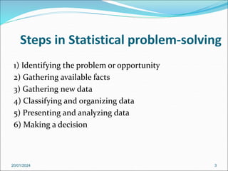
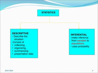
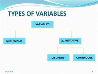
1. INTRODUCTION TO STATISTICS
20/01/2024 1

2. NATURE OF STATISTICS
 STATISTICS – scientific procedures and methods for collecting,
organising, summarising, presenting and analysing data, as
well as obtaining useful information, drawing valid conclusions
and making effective decisions based on the analysis.
 Example :
 Public health : an administrator might be concerned with the
number of resident contract a new flu virus during a certain year
 Education : a researcher might want to know if methods of
teaching are better than olds one
20/01/2024 2

3. Steps in Statistical problem-solving
1) Identifying the problem or opportunity
2) Gathering available facts
3) Gathering new data
4) Classifying and organizing data
5) Presenting and analyzing data
6) Making a decision
20/01/2024 3

4. 20/01/2024
STATISTICS
DESCRIPTIVE
- Describe the
situation
-Consist of
• collecting,
• organizing,
• summarizing
• presentation data
INFERENTIAL
-make inference
from samples to
populations
- uses probability
4

5. TERM IN STATISTICS
 Population : consists of all subjects (human or otherwise)
that are being studied
 Sample : group of subjects selected from population
 Statistic – summary measure computed from sample data
 Parameter – summary measure for the entire population
 Census – if the study is carried out using the whole
population
 Sample survey – involved a subgroup (or sample) of a
population being chosen
 Pilot study – is a study done before the actual fieldwork is
carried out.
20/01/2024 5

6. Data
 Primary data
 Data collected from primary source or from sample
 Example : interviews the respondents, distribute
questionnaire
 Advantages –
1) more accurate and consistent
2)Able to explain how the data are collected
 Disadvantages -
1) Requires more time, manpower, high cost
20/01/2024 6

7.  Secondary Data
 Data collected from other parties
 Example : Bank Negara, Statistics Department
 Advantage
1) easily accessible from the internet, journals,
annual report etc.
2) inexpensive, less time to collect
 Disadvantage
1) lack accuracy because method of data collection
are not explained
2) biased – original purpose of data collection is not
known
3) not meet the specific needs and objectives
20/01/2024 7

8. TYPES OF VARIABLES
20/01/2024
VARIABLES
QUALITATIVE QUANTITATIVE
DISCRETE CONTINUOUS
8

9.  Qualitative : variable that can categorize according to
some characteristic or attribute.
Example : gender (male or female), religious preference
(Muslim, Buddha, Christian)
 Quantitative : numerical and can be order or rank.
Example : Age, height, body temperature
20/01/2024 9

10.  Discrete : assume value that can be counted. 0, 1, 2, 3, …
Example : number of children in a family, number of
student in a classroom.
 Continuous : assume an infinite number of values
between any two specific values. Usually obtained by
measuring. Include fractions and decimals
Example : weight, height, time, mass, etc.
20/01/2024 10

11. Scale of measurement
 Nominal scale – categorical data
o The number in the data cannot be added or subtracted
from another number.
o Example: gender (male, female), religion (muslim,
christian, hinduism)
 Ordinal scale – can be arranged in ranking order and
inequality signs can be used when comparing the value of
the variable.
o Example: size of building (small, medium, large),
education level (Phd, Master, Degree, Diploma)
20/01/2024 11

12. Cont..
 Interval scale – the differences between data value are
meaningful but cannot be manipulated with multiplication
and division.
o Example: IQ score, temperature
 Ratio scale – is the interval measurement with an inherent
zero setting.
o Example: height, weight, time taken to complete a given
task, monthly income.
20/01/2024 12

13. SAMPLING AND DATA COLLECTION METHODS
20/01/2024 13

14. Non-Probability Sampling Techniques
 Convenience sampling
pre-testing of questionnaires
 Judgemental Sampling
selected based on the judgement
 Snowball Sampling
select respondent at random. After interviewed, asked
respondent to identify others who are in the target
population of interest
 Quota Sampling
observes the specific characteristics of potential
respondent.
20/01/2024 14

15.  Simple random sampling
each item have the same chance of being selected as a
sample
 Systematic sampling
Samples are selected by using every kth number after the
first subject is randomly selected from 1 through k
20/01/2024 15
Probability Sampling Techniques

16.  Stratified sampling
divide the population into groups (strata) and samples selected
randomly within groups
 Example:
A factory manager wants to find out what his workers think about the
factory canteen facilities. He decides to give a questionnaire to a sample
of 80 workers. It is though that different age groups will have different
opinions.
There are 75 workers between 18 and 32, 140 workers between 33 and 47
and 85 workers between 48 and 62.
20/01/2024 16
Probability Sampling Techniques

17.  Cluster
divide population into subpopulations or clusters.
 Multi-stage sampling
This method is designed to reduce time and cost when
working with samples from very large populations.
20/01/2024 17
Probability Sampling Techniques

18. Data Collection Methods
 Face-to-face interview
 Telephone interview
 Direct questionnaire
 Mail (or postal) questionnaire
 Direct observation
20/01/2024 18

19. Designing a questionnaire
In designing a questionnaire, the following points
should be taken into consideration.
 The questionnaire should be short and simple
 Begin with simple and less controversial questions first
 Should not be biased towards certain groups
 Avoid sensitive questions
 A questionnaire checklist can be constructed to ensure
all required data are included.
20/01/2024 19
iam/ppssp/fskm/2013

20. DATA PRESENTATION
20/01/2024 20

21. Organizing and graphing qualitative data
Example 1
Twenty-five army inductees were given a blood test to
determine their blood type. The data set is
A B B AB O
O O B AB B
B B O A O
A O O O AB
AB A O B A
Construct a frequency distribution for the data
20/01/2024 21
1)Frequency distribution

22. Blood type Frequency
A
B
O
AB
20/01/2024 22

23. 2) Pie Chart
 A pie graph is a circle that is divided into sections or
wedges according to the percentage of frequencies in
each category of the distribution.
 Procedure for constructing a pie chart : Refer to
Example 1
Step 1: Number of categories = 4
20/01/2024 23

24.  Step 2 : Percentage
 Step 3 : Convert to degrees (total 360)
%
16
100
25
4
:
%
36
100
25
9
:
%
28
100
25
7
:
%
20
100
25
5
:








AB
O
B
A
20/01/2024 24
100


n
f
o
o
o
o
o
o
o
o
AB
O
B
A
6
.
57
360
%
16
:
6
.
129
360
%
36
:
8
.
100
360
%
28
:
72
360
%
20
:









25. 20/01/2024 25

26. 3) Bar Chart
 A graph of bars whose heights represent the
frequencies of respective categories
 Categories on the vertical axis
 Frequencies on the horizontal axis.
20/01/2024 26

27. Vertical bar chart
20/01/2024 27

28. 3a) Cluster/multiple bar chart
No College Four-year degree Advanced Degree
Urban 15 12 8
Suburban 8 15 9
Rural 6 8 7
0
2
4
6
8
10
12
14
16
20/01/2024 28

29. 3b) Stacked/component bar chart
Example 2
 A random sample of car owners was selected and the
following results were obtained.
20/01/2024 29
Car ownership City Town Rural
Owns a foreign car 90 60 25
Do not own a foreign car 110 90 125
Total 200 150 150

30. Solution
% of car ownership City Town Rural
Owns a foreign car 45 40 16.7
Do not own a foreign car 55 60 83.3
Total 100 100 100
20/01/2024 30
0%
20%
40%
60%
80%
100%
City Town Rural
Percentage of car ownership
Do not own a
foreign car
Owns a foreign
car

31. 4) Contingency table
 Also known as cross tabulation.
 To examine the categorical responses in term of two
qualitative variables simultaneously.
20/01/2024 31
Red Green White Black Total
Men 30 10 26 34 100
Women 8 10 45 37 100
Total 75 18 63 44 200

32. 2-32
1) Stem-and-Leaf Plots
 This plot separates data entries into leading digits and
trailing digits.
 Steps
a) Split each value into two sets of digits.
b) List all the possible stem digits from the lowest to the
highest.
c) For each score in the mass of data, write down the leaf
numbers on the line labelled by the appropriate stem
number.
20/01/2024
Organizing and graphing quantitative data

33. Example 3
 Display the following data with a stem-and-leaf plot.
3.4 4.5 2.3 2.7 3.8 5.9 3.4 4.7 2.4 4.1 3.6 5.1
20/01/2024 33

34. Example 4
 Construct a stem and leaf plot by using classes 0-4, 5-9,
10-14, 15-19, and 20-24
20/01/2024 34
3 9 14 22 11 4 12 0
15 20 8 7 5 1 7 13
9 8 14 11 19 17 3 6

35. 2) Histogram
 Histogram – graph that
displays the data by using
contiguous vertical bars
(unless the frequency of a
class is 0) of various
heights to represent the
frequencies of the classes.
0
2
4
6
8
0 10.5 20.5 30.5 40.5 50.5 60.5 70.5 80.5
Class Boundaries
Frequency
20/01/2024 35

36. Example 5
 The table below shows the weight of 100 honeydews
produced from Farm X. Draw a histogram representing
the weight distribution of the honeydews.
20/01/2024 36
Weight (‘00 g) Frequency
4 – 6 4
6 – 8 9
8 – 10 34
10 – 12 25
12 - 14 28

37. 3) Frequency polygon
 If a histogram is available, the frequency polygon is
obtained by connecting the mid-point of the tops of
the rectangles in the histogram.
20/01/2024 37

38. 4) Cumulative frequency distribution
and ogives
 Cumulative frequency distribution
There are 2 types of cumulative frequency distributions. They
are ‘less than’ and ‘more than’ cumulative distribution. The
‘less than’ cumulative frequency is more frequently used.
 Ogives (Cumulative frequency curve)
Ogive is a graph or line chart of a cumulative frequency
distribution. There are 2 types of ogives. They are ‘less than’
ogive and ‘more than’ ogive.
20/01/2024 38

39.  Example 6
 The table below shows the number of service years of 120
employees at a firm called SITI. Draw a ‘less than’ ogive.
20/01/2024 39
Service years No of employees
1 – 4 16
5 – 8 20
9 – 12 28
13 – 16 24
17 – 20 16
21 – 24 11
25 – 28 5

40.  Solution
20/01/2024 40
Service years Cumulative frequency
Less than 0.5 0
Less than 4.5 16
Less than 8.5 36
Less than 12.5 64
Less than 16.5 88
Less than 20.5 104
Less than 24.5 115
Less than 28.5 120

41. 20/01/2024 41