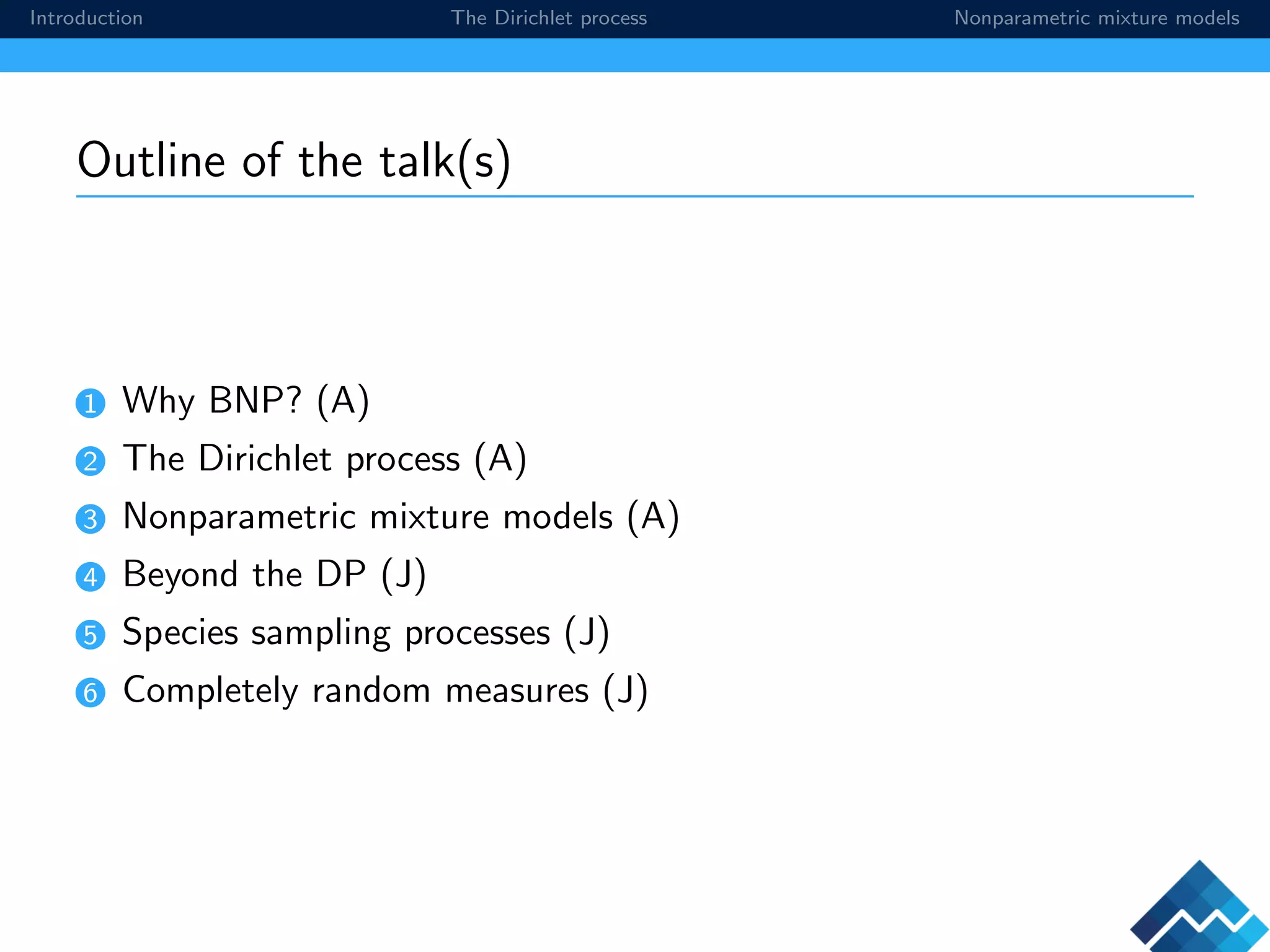
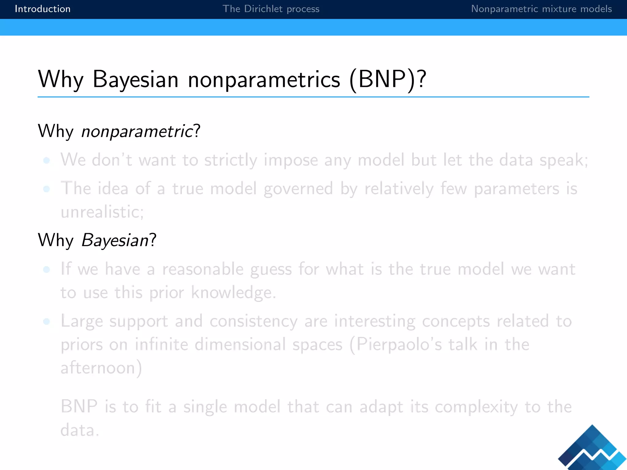
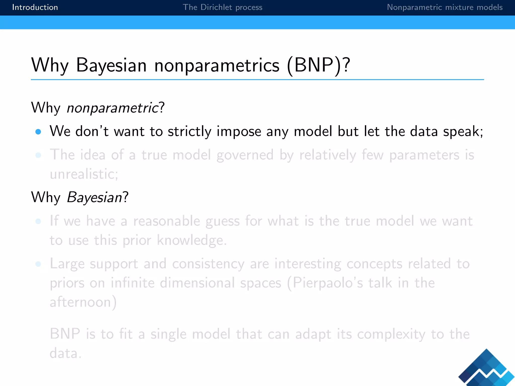
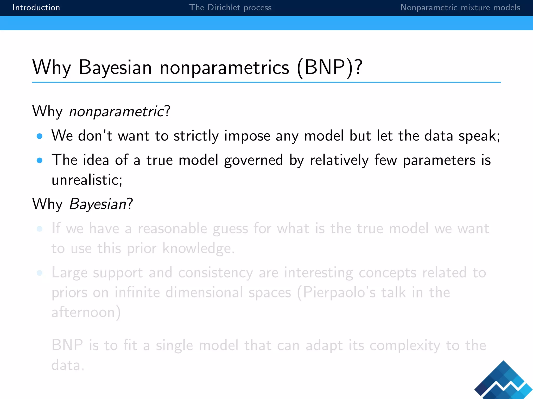
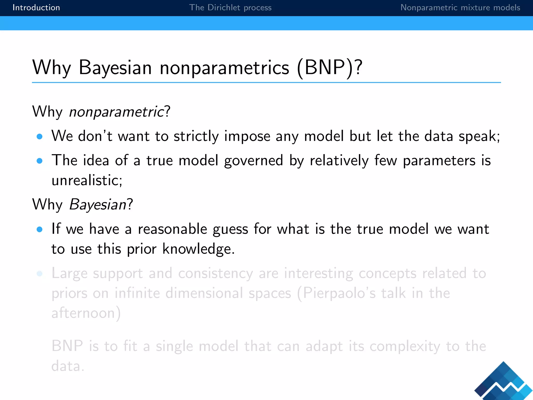
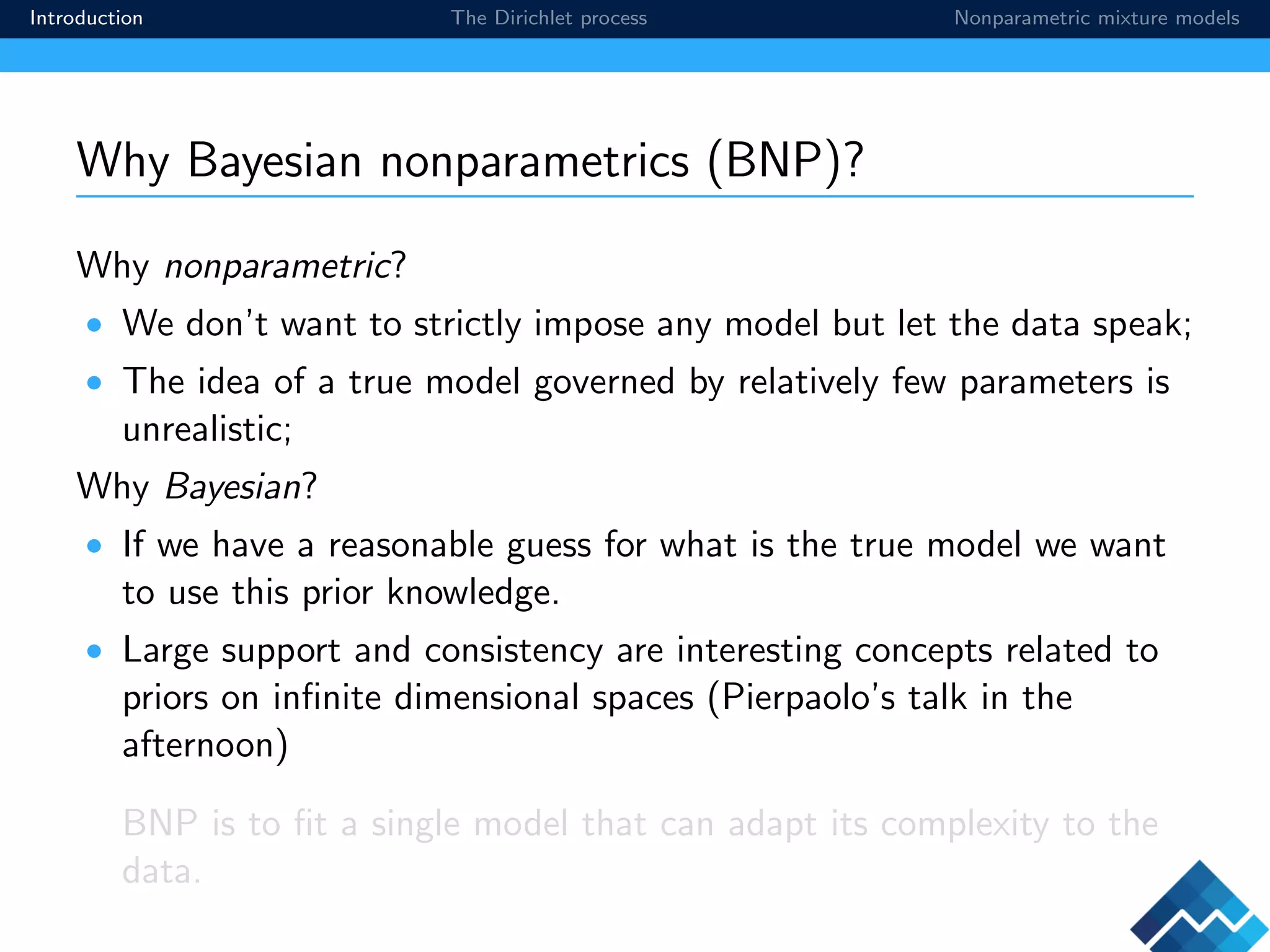
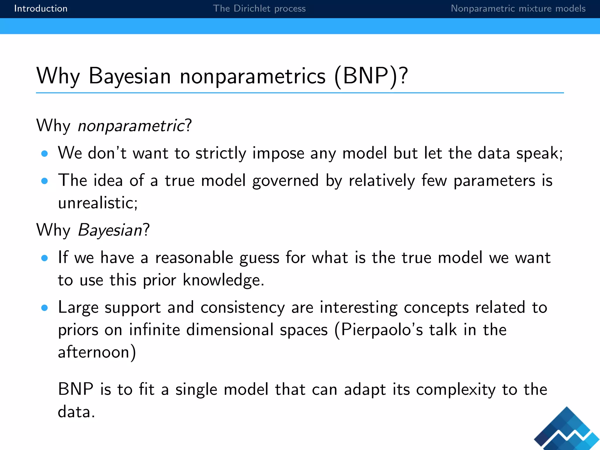
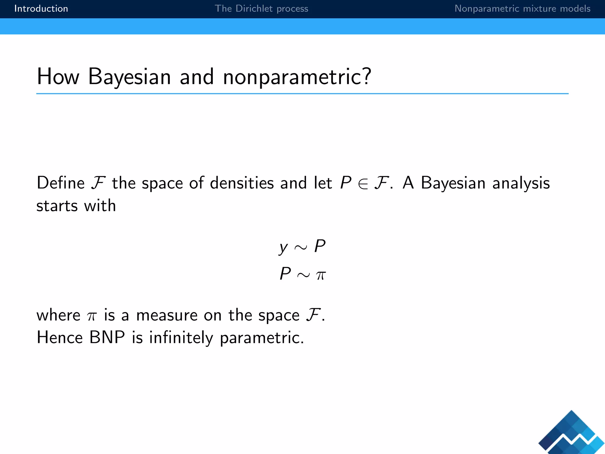
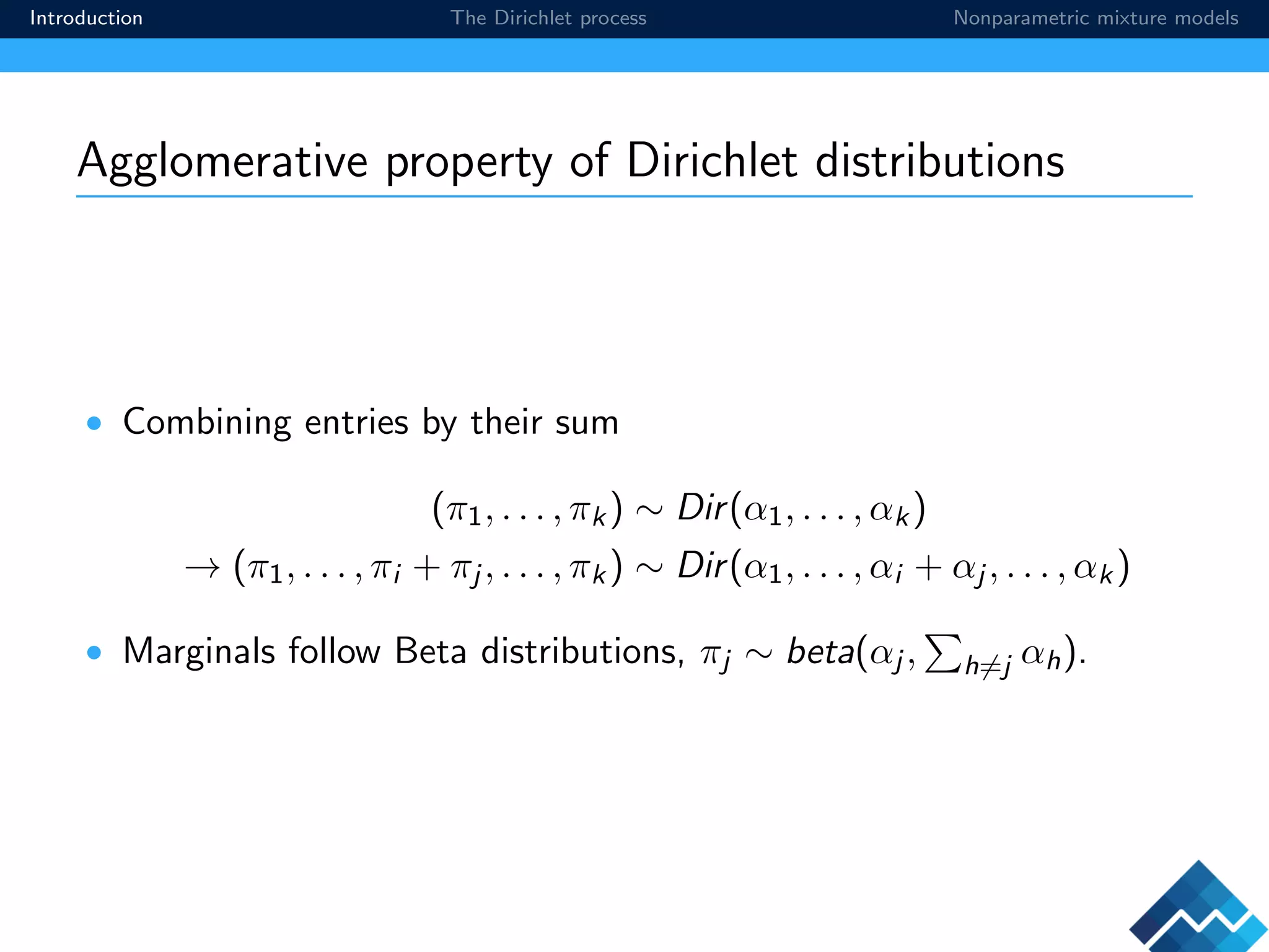
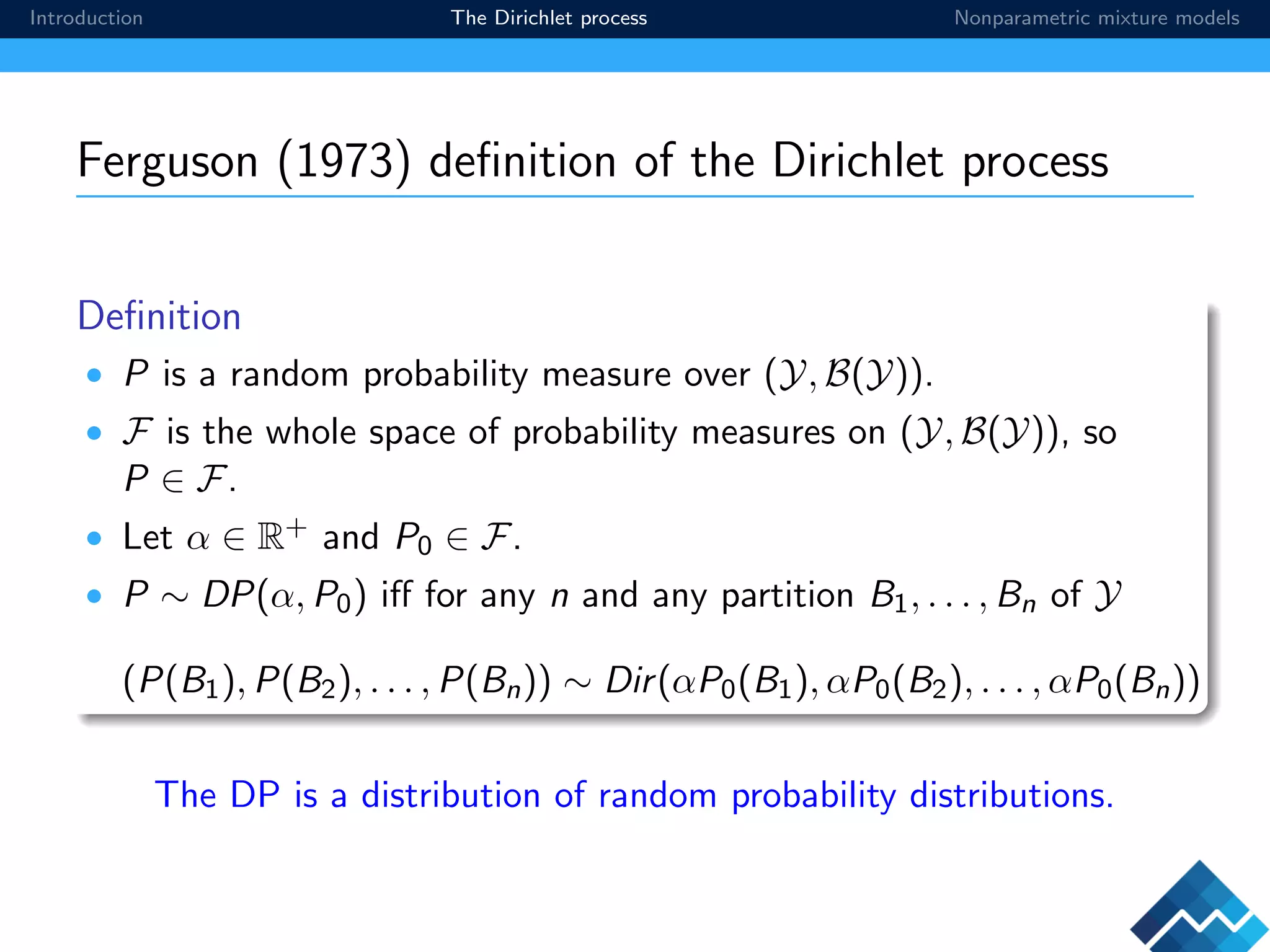
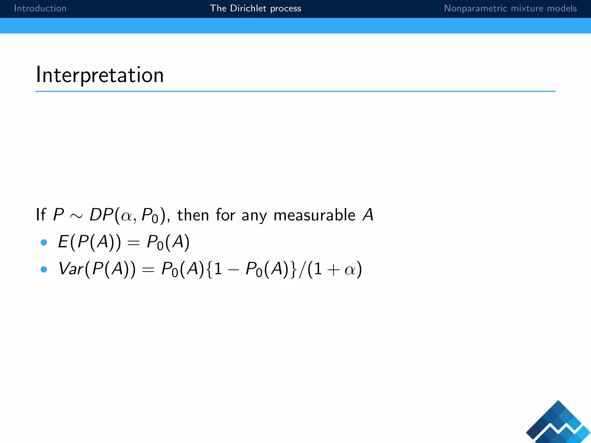
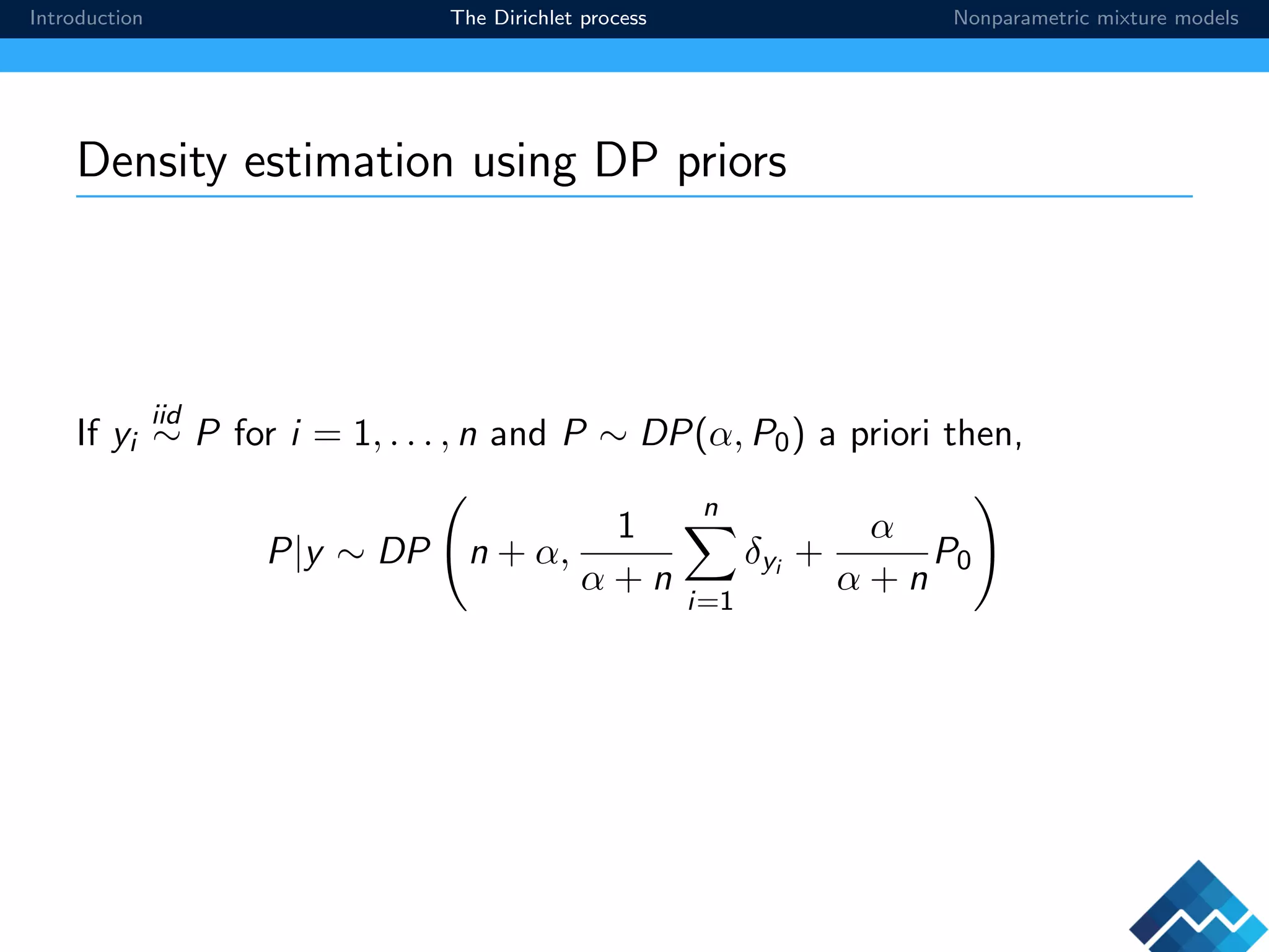
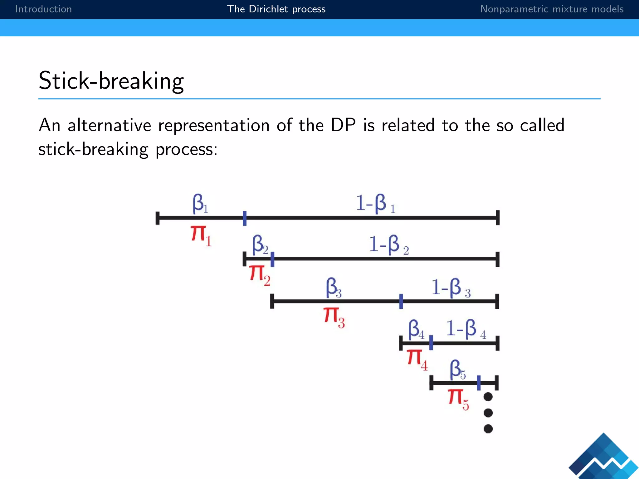
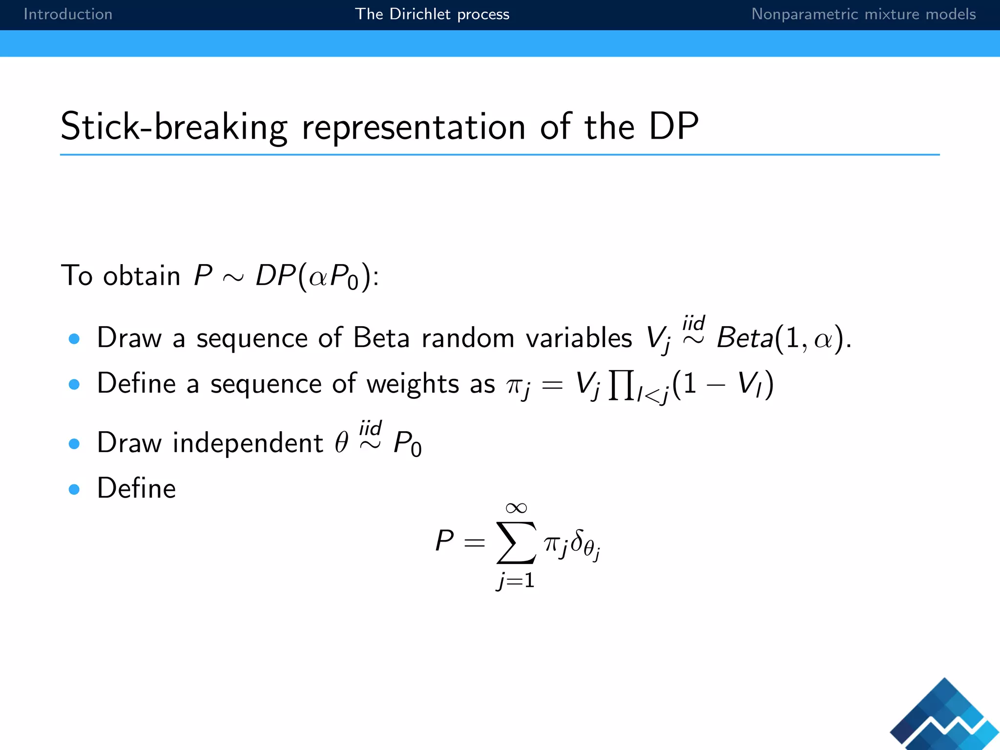
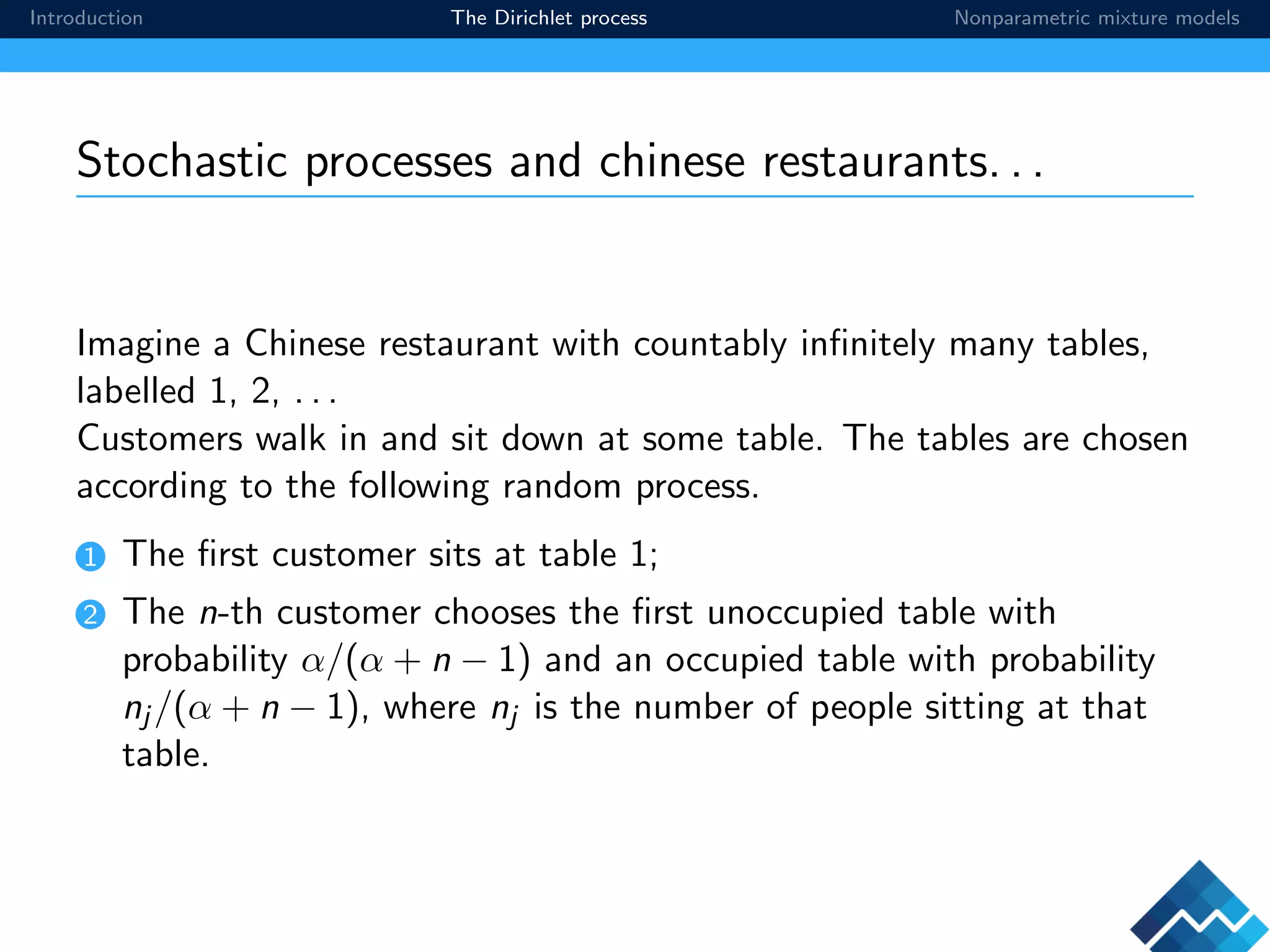
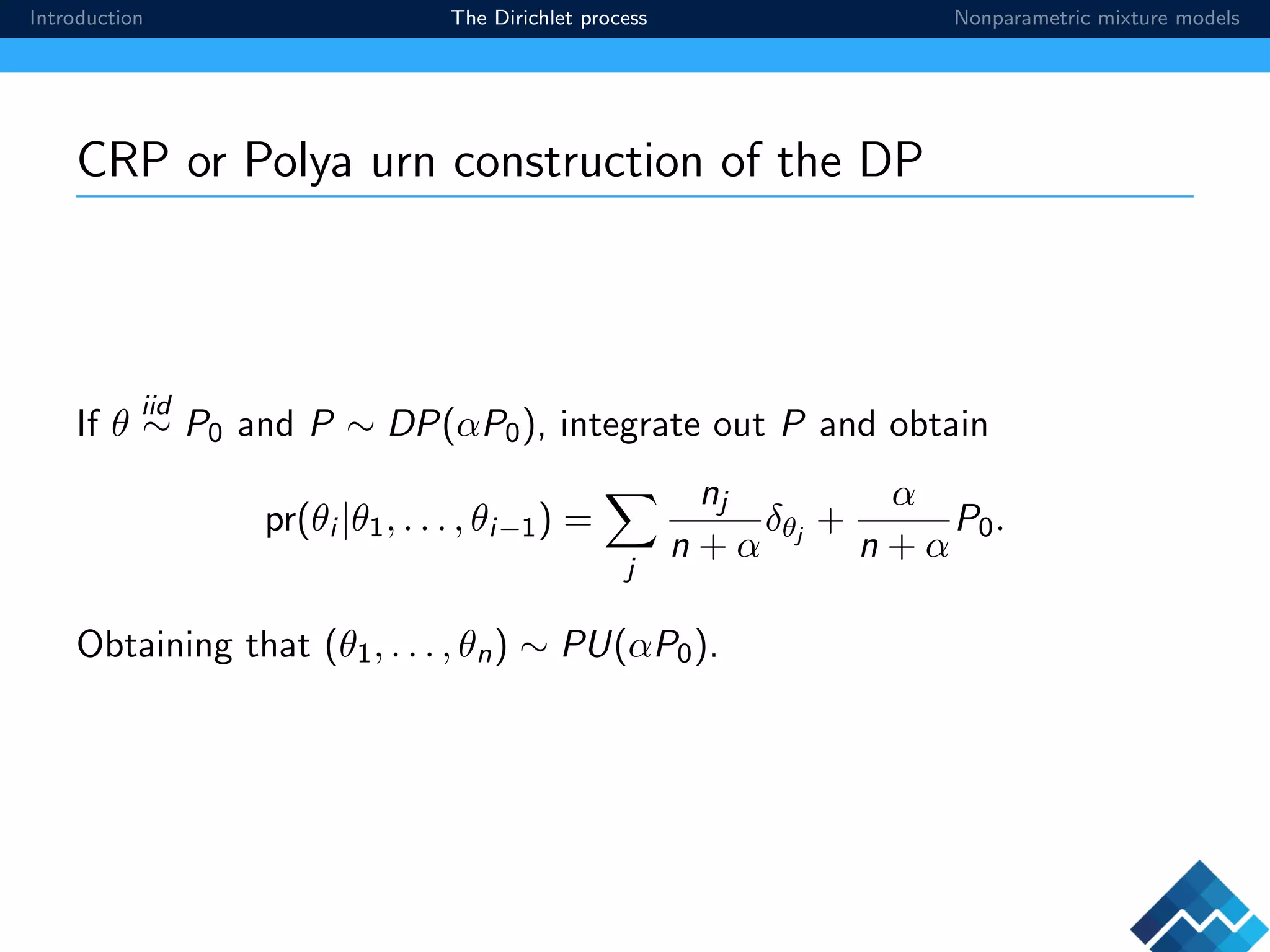
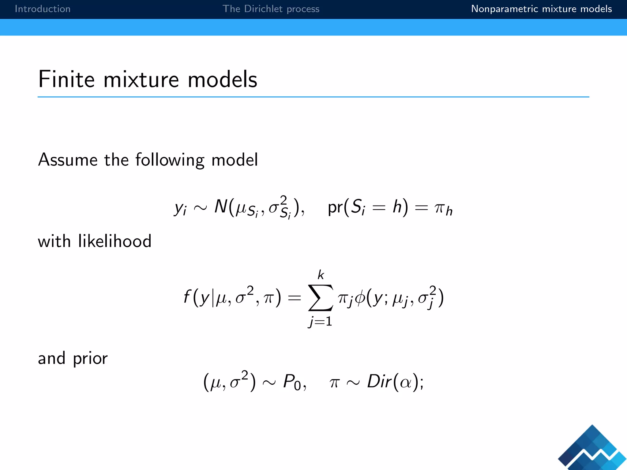
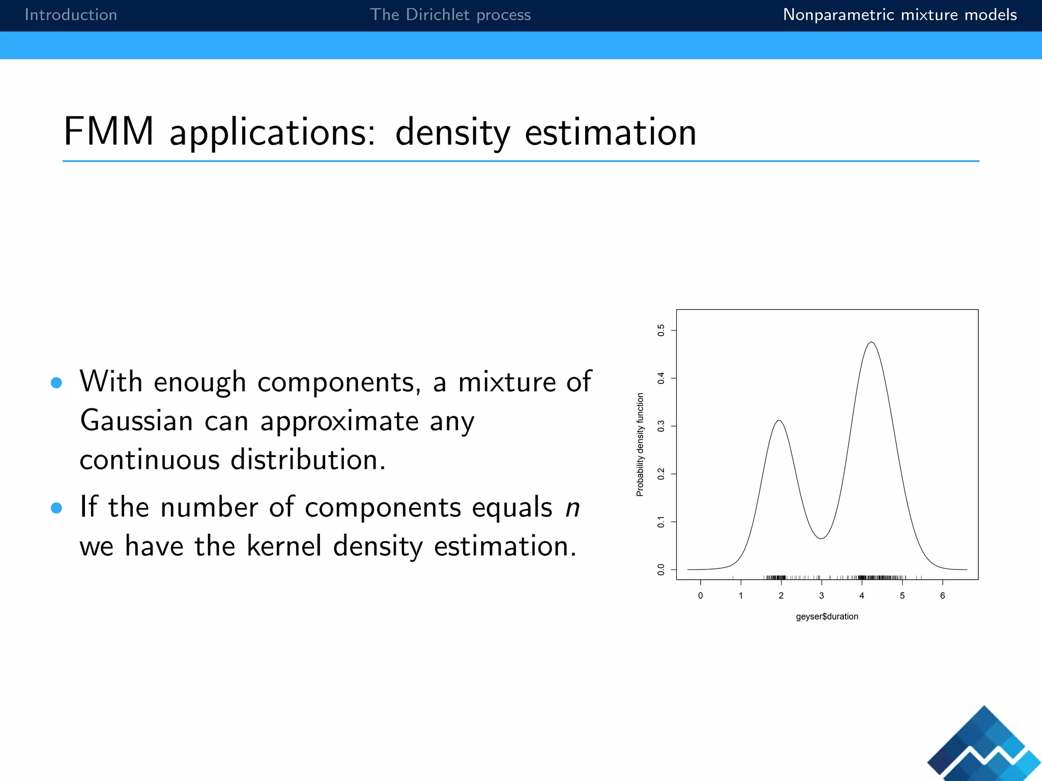
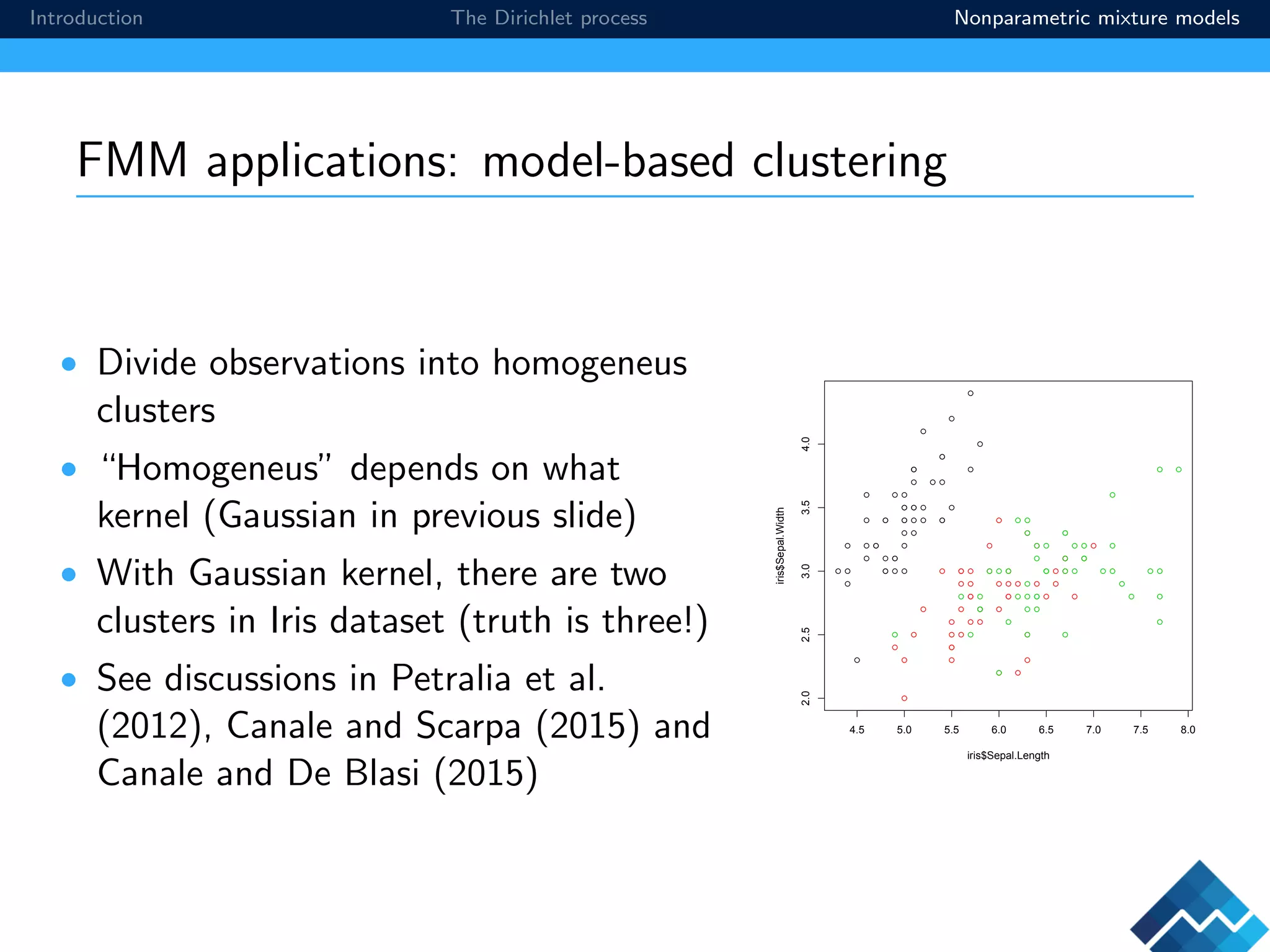
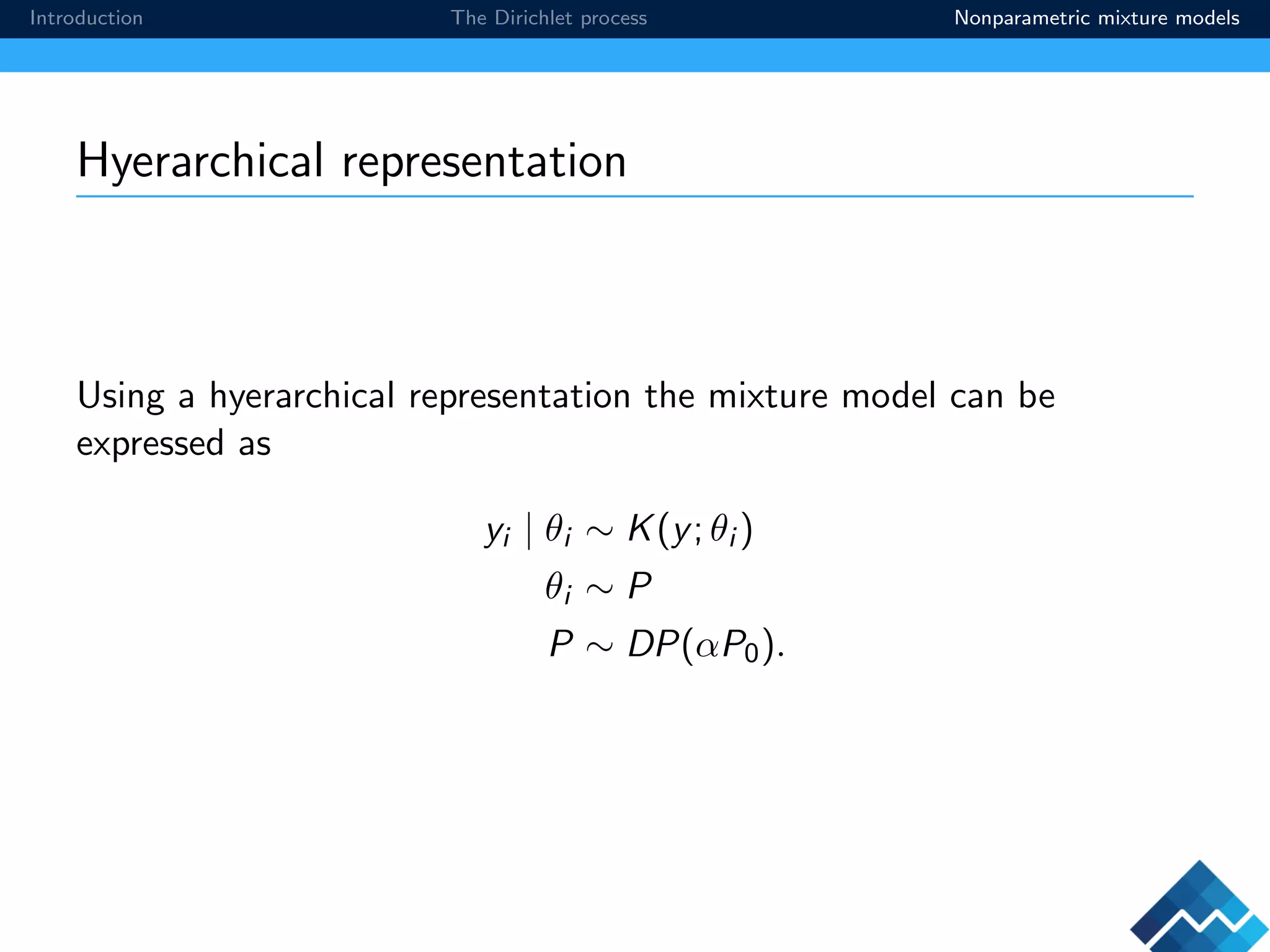
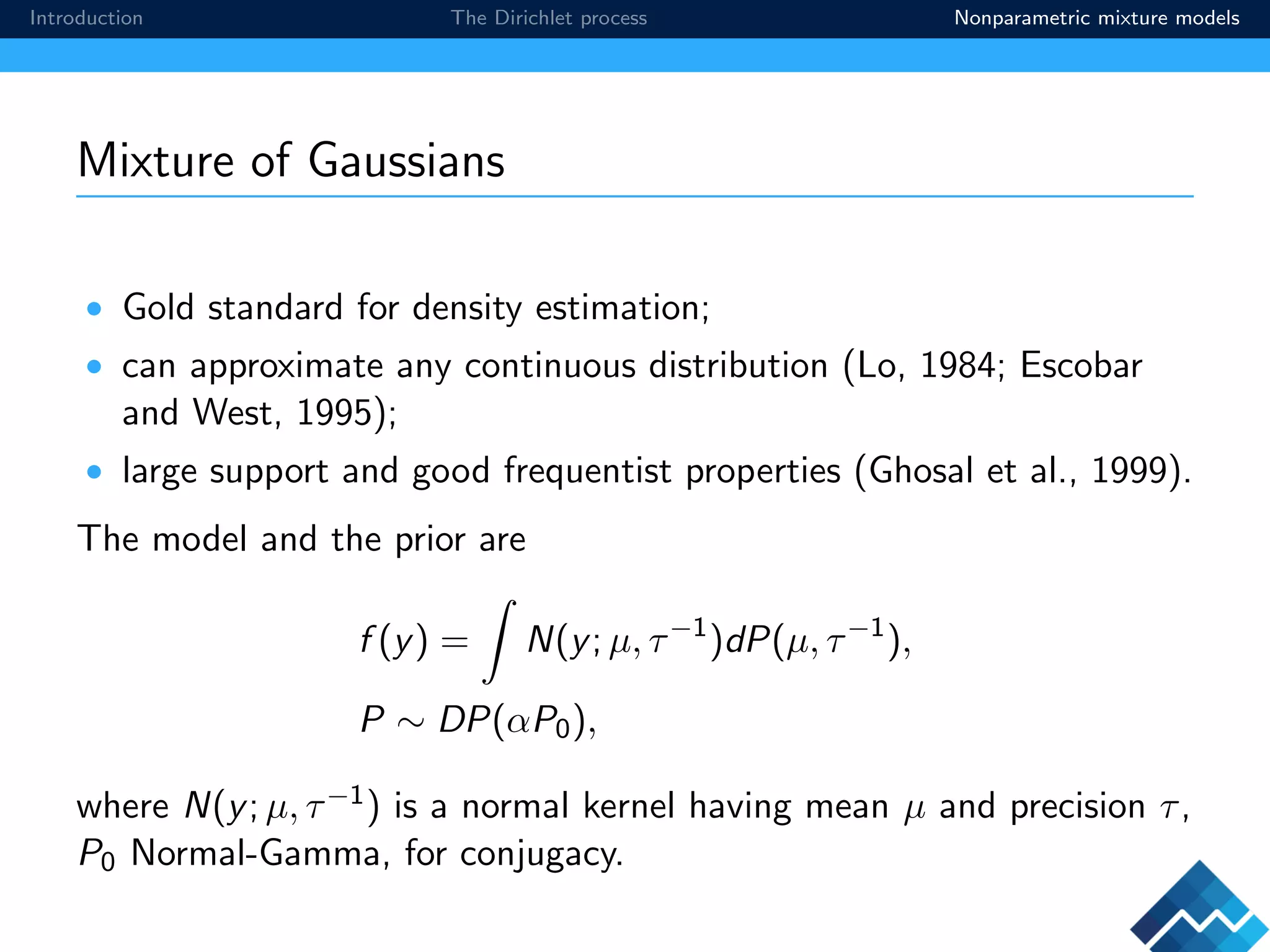
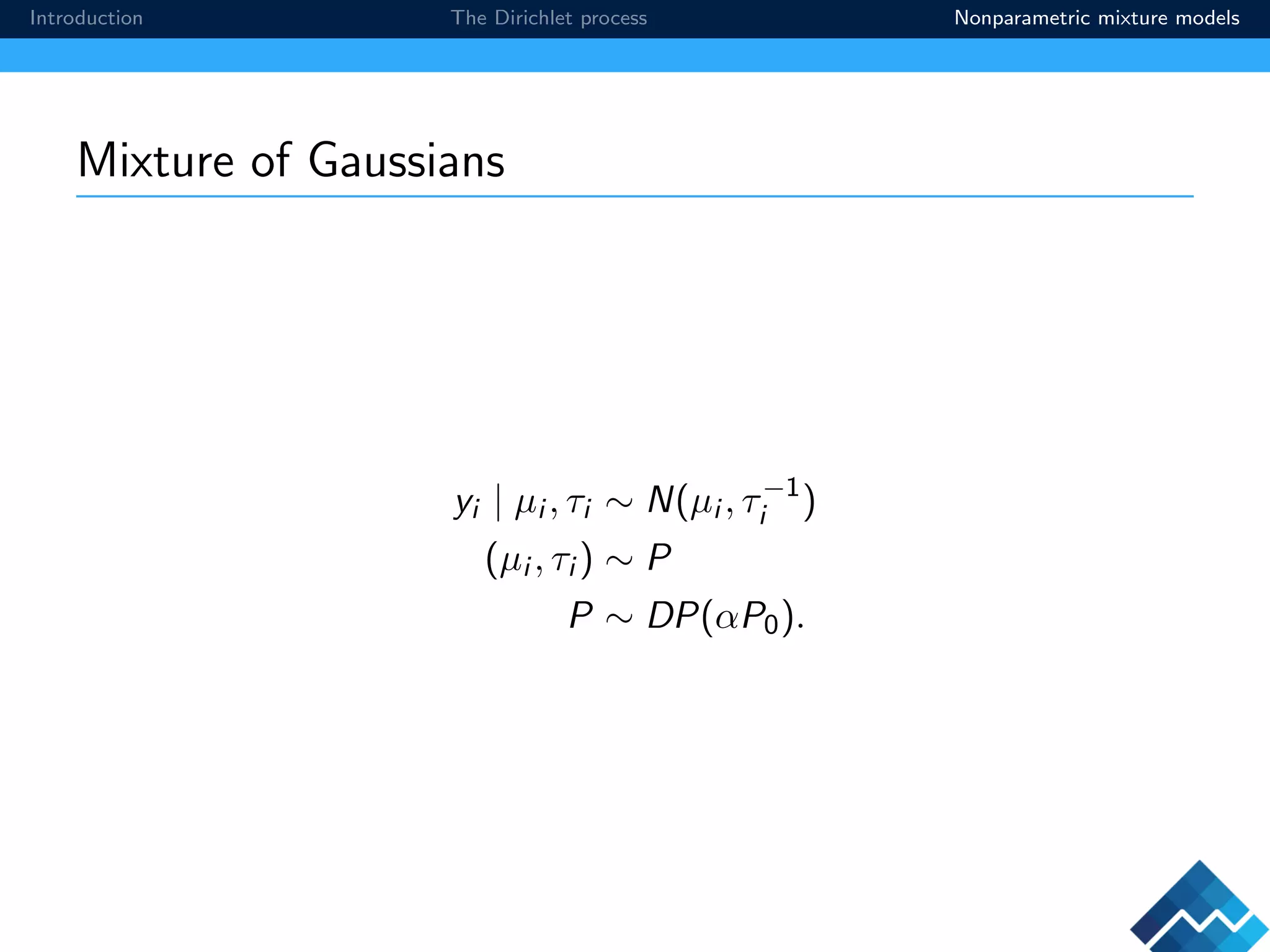
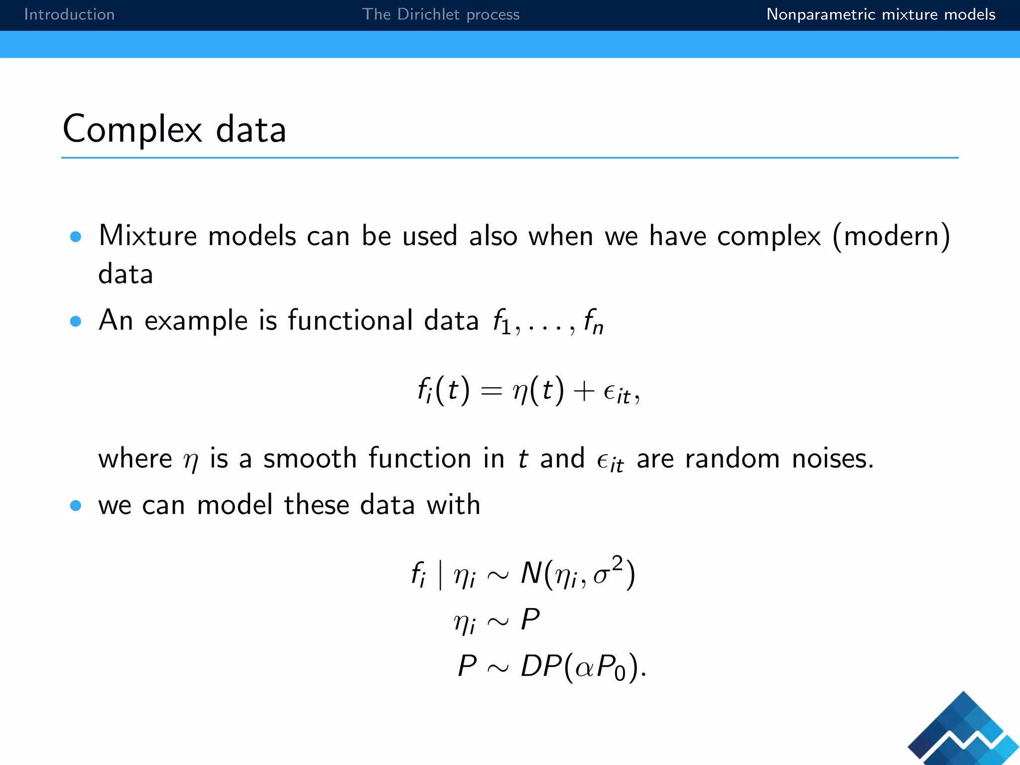
The document provides an introduction to Bayesian nonparametrics and the Dirichlet process. It explains that Bayesian nonparametrics aims to fit models that can adapt their complexity based on the data, without strictly imposing a fixed structure. The Dirichlet process is described as a prior distribution on the space of all probability distributions, allowing the model to utilize an infinite number of parameters. Nonparametric mixture models using the Dirichlet process provide a flexible approach to density estimation and clustering.

1. A gentle introduction to BNP
Part I
Antonio Canale
Universit`a di Torino &
Collegio Carlo Alberto
StaTalk on BNP, 19/02/16

2. Introduction The Dirichlet process Nonparametric mixture models
Outline of the talk(s)
1 Why BNP? (A)
2 The Dirichlet process (A)
3 Nonparametric mixture models (A)
4 Beyond the DP (J)
5 Species sampling processes (J)
6 Completely random measures (J)

3. Introduction The Dirichlet process Nonparametric mixture models
Why Bayesian nonparametrics (BNP)?
Why nonparametric?
• We don’t want to strictly impose any model but let the data speak;
• The idea of a true model governed by relatively few parameters is
unrealistic;
Why Bayesian?
• If we have a reasonable guess for what is the true model we want
to use this prior knowledge.
• Large support and consistency are interesting concepts related to
priors on infinite dimensional spaces (Pierpaolo’s talk in the
afternoon)
BNP is to fit a single model that can adapt its complexity to the
data.

4. Introduction The Dirichlet process Nonparametric mixture models
Why Bayesian nonparametrics (BNP)?
Why nonparametric?
• We don’t want to strictly impose any model but let the data speak;
• The idea of a true model governed by relatively few parameters is
unrealistic;
Why Bayesian?
• If we have a reasonable guess for what is the true model we want
to use this prior knowledge.
• Large support and consistency are interesting concepts related to
priors on infinite dimensional spaces (Pierpaolo’s talk in the
afternoon)
BNP is to fit a single model that can adapt its complexity to the
data.

5. Introduction The Dirichlet process Nonparametric mixture models
Why Bayesian nonparametrics (BNP)?
Why nonparametric?
• We don’t want to strictly impose any model but let the data speak;
• The idea of a true model governed by relatively few parameters is
unrealistic;
Why Bayesian?
• If we have a reasonable guess for what is the true model we want
to use this prior knowledge.
• Large support and consistency are interesting concepts related to
priors on infinite dimensional spaces (Pierpaolo’s talk in the
afternoon)
BNP is to fit a single model that can adapt its complexity to the
data.

6. Introduction The Dirichlet process Nonparametric mixture models
Why Bayesian nonparametrics (BNP)?
Why nonparametric?
• We don’t want to strictly impose any model but let the data speak;
• The idea of a true model governed by relatively few parameters is
unrealistic;
Why Bayesian?
• If we have a reasonable guess for what is the true model we want
to use this prior knowledge.
• Large support and consistency are interesting concepts related to
priors on infinite dimensional spaces (Pierpaolo’s talk in the
afternoon)
BNP is to fit a single model that can adapt its complexity to the
data.

7. Introduction The Dirichlet process Nonparametric mixture models
Why Bayesian nonparametrics (BNP)?
Why nonparametric?
• We don’t want to strictly impose any model but let the data speak;
• The idea of a true model governed by relatively few parameters is
unrealistic;
Why Bayesian?
• If we have a reasonable guess for what is the true model we want
to use this prior knowledge.
• Large support and consistency are interesting concepts related to
priors on infinite dimensional spaces (Pierpaolo’s talk in the
afternoon)
BNP is to fit a single model that can adapt its complexity to the
data.

8. Introduction The Dirichlet process Nonparametric mixture models
Why Bayesian nonparametrics (BNP)?
Why nonparametric?
• We don’t want to strictly impose any model but let the data speak;
• The idea of a true model governed by relatively few parameters is
unrealistic;
Why Bayesian?
• If we have a reasonable guess for what is the true model we want
to use this prior knowledge.
• Large support and consistency are interesting concepts related to
priors on infinite dimensional spaces (Pierpaolo’s talk in the
afternoon)
BNP is to fit a single model that can adapt its complexity to the
data.

9. Introduction The Dirichlet process Nonparametric mixture models
How Bayesian and nonparametric?
Define F the space of densities and let P ∈ F. A Bayesian analysis
starts with
y ∼ P
P ∼ π
where π is a measure on the space F.
Hence BNP is infinitely parametric.

10. Introduction The Dirichlet process Nonparametric mixture models
The Dirichlet distribution
• Start with independent Zj ∼ Ga(αj , 1), for j = 1, . . . , k (αj > 0)
• Define
πj =
Zj
k
j=1 Zj
;
• Then (π1, . . . , πk) ∼ Dir(α1, . . . , αk);
• The Dirichlet distribution is a distribution over the K-dimensional
probability simplex:
∆k = {(π1, . . . , πk) : πj > 0,
j
πj = 1}

11. Introduction The Dirichlet process Nonparametric mixture models
The Dirichlet distribution
• Probability density
p(π1, . . . , πk|α) =
Γ( j αj )
j Γ(αj )
j
π
αj −1
j

12. Introduction The Dirichlet process Nonparametric mixture models
The Dirichlet distribution in Bayesian statistics
Dirichlet distribution is conjugate to the multinomial likelihood, hence
if
π ∼ Dir(α)
y|π ∼ Multinomial(π)
p(y = j|π) = πj ,
then we have
p(π|y = j, α) = Dir(ˆα)
where ˆαj = αj + 1, ˆαi = αi for each i = j.

13. Introduction The Dirichlet process Nonparametric mixture models
Agglomerative property of Dirichlet distributions
• Combining entries by their sum
(π1, . . . , πk) ∼ Dir(α1, . . . , αk)
→ (π1, . . . , πi + πj , . . . , πk) ∼ Dir(α1, . . . , αi + αj , . . . , αk)
• Marginals follow Beta distributions, πj ∼ beta(αj , h=j αh).

14. Introduction The Dirichlet process Nonparametric mixture models
1 Introduction
2 The Dirichlet process
3 Nonparametric mixture models

15. Introduction The Dirichlet process Nonparametric mixture models
Ferguson (1973) definition of the Dirichlet process
Definition
• P is a random probability measure over (Y, B(Y)).
• F is the whole space of probability measures on (Y, B(Y)), so
P ∈ F.
• Let α ∈ R+ and P0 ∈ F.
• P ∼ DP(α, P0) iff for any n and any partition B1, . . . , Bn of Y
(P(B1), P(B2), . . . , P(Bn)) ∼ Dir(αP0(B1), αP0(B2), . . . , αP0(Bn))
The DP is a distribution of random probability distributions.

16. Introduction The Dirichlet process Nonparametric mixture models
Interpretation
If P ∼ DP(α, P0), then for any measurable A
• E(P(A)) = P0(A)
• Var(P(A)) = P0(A){1 − P0(A)}/(1 + α)

17. Introduction The Dirichlet process Nonparametric mixture models
Density estimation using DP priors
If yi
iid
∼ P for i = 1, . . . , n and P ∼ DP(α, P0) a priori then,
P|y ∼ DP n + α,
1
α + n
n
i=1
δyi +
α
α + n
P0

18. Introduction The Dirichlet process Nonparametric mixture models
Density estimation using DP priors
−6 −4 −2 0 2 4 6
0.00.20.40.60.81.0
x
−6 −4 −2 0 2 4 6
0.00.20.40.60.81.0
x
Figure: Black true density (N(1, 2)), blue base measure (N(0,1)), green
dashed ECDF, blue dashed posterior DP. First plot n = 10, second n = 50.

19. Introduction The Dirichlet process Nonparametric mixture models
Stick-breaking
An alternative representation of the DP is related to the so called
stick-breaking process:

20. Introduction The Dirichlet process Nonparametric mixture models
Stick-breaking representation of the DP
To obtain P ∼ DP(αP0):
• Draw a sequence of Beta random variables Vj
iid
∼ Beta(1, α).
• Define a sequence of weights as πj = Vj l<j (1 − Vl )
• Draw independent θ
iid
∼ P0
• Define
P =
∞
j=1
πj δθj

21. Introduction The Dirichlet process Nonparametric mixture models
Stochastic processes and chinese restaurants. . .
Imagine a Chinese restaurant with countably infinitely many tables,
labelled 1, 2, . . .
Customers walk in and sit down at some table. The tables are chosen
according to the following random process.
1 The first customer sits at table 1;
2 The n-th customer chooses the first unoccupied table with
probability α/(α + n − 1) and an occupied table with probability
nj /(α + n − 1), where nj is the number of people sitting at that
table.

22. Introduction The Dirichlet process Nonparametric mixture models
CRP or Polya urn construction of the DP
If θ
iid
∼ P0 and P ∼ DP(αP0), integrate out P and obtain
pr(θi |θ1, . . . , θi−1) =
j
nj
n + α
δθj
+
α
n + α
P0.
Obtaining that (θ1, . . . , θn) ∼ PU(αP0).

23. Introduction The Dirichlet process Nonparametric mixture models
Considerations
• Draw from a DP are a.s. discrete
• Unappealing if y is continuous, useful if y is discrete? (no, but
wait for my afternoon talk)

24. Introduction The Dirichlet process Nonparametric mixture models
Considerations
• Draw from a DP are a.s. discrete
• Unappealing if y is continuous, useful if y is discrete? (no, but
wait for my afternoon talk)

25. Introduction The Dirichlet process Nonparametric mixture models
Finite mixture models
Assume the following model
yi ∼ N(µSi
, σ2
Si
), pr(Si = h) = πh
with likelihood
f (y|µ, σ2
, π) =
k
j=1
πj φ(y; µj , σ2
j )
and prior
(µ, σ2
) ∼ P0, π ∼ Dir(α);

26. Introduction The Dirichlet process Nonparametric mixture models
FMM applications: density estimation
• With enough components, a mixture of
Gaussian can approximate any
continuous distribution.
• If the number of components equals n
we have the kernel density estimation.
0 1 2 3 4 5 6
0.00.10.20.30.40.5
geyser$duration
Probabilitydensityfunction

27. Introduction The Dirichlet process Nonparametric mixture models
FMM applications: model-based clustering
• Divide observations into homogeneus
clusters
• “Homogeneus” depends on what
kernel (Gaussian in previous slide)
• With Gaussian kernel, there are two
clusters in Iris dataset (truth is three!)
• See discussions in Petralia et al.
(2012), Canale and Scarpa (2015) and
Canale and De Blasi (2015)
q
q
q
q
q
q
q q
q
q
q
q
qq
q
q
q
q
qq
q
q
q
q
q
q
q
q
q
q
q
q
q
q
q
q
q
q
q
q
q
q
q
q
q
q
q
q
q
q
qq
q
q
qq
q
q
q
q
q
q
q
qq
q
q
q
q
q
q
q
q
q
q
q
q
q
q
q
qq
q q
q
q
q
q
q
q
q
q
q
q
q
q
q q
q
q
q
q
q
q
q q
q
q
q
q
q
q
q
q
q
q
q
q
q
q
q
q q
q
q
q
q
q
q
q
q
q
qq
q
q
q
q
q
qq q
q
q
q
q
q
q
q
q
4.5 5.0 5.5 6.0 6.5 7.0 7.5 8.0
2.02.53.03.54.0
iris$Sepal.Length
iris$Sepal.Width

28. Introduction The Dirichlet process Nonparametric mixture models
Infinite mixture models
• A more elegant way to write the finite mixture model is
f (y) = K(y; θ)dP(θ), P =
K
j=1
ωj δθj
,
where K(·; θ) is a general kernel (e.g. normal) parametrized by θ.
• Clearly a prior on the weights and on the parameters of the kernel
is equivalent to a prior on the finite disrete measure P.
• From FMM to IMM ⇒ P ∼ DP(αP0)!

29. Introduction The Dirichlet process Nonparametric mixture models
DP mixture models
• The model and prior are
y ∼ f , f (y) = K(y; θ)dP(θ), P ∼ DP(αP0).
where K(·; θ) is a general kernel (e.g. normal) parametrized by θ.
• Consider the DPM prior as a “smoothed version” of the DP prior
(just like the kernel density estimation is a smoothed version of the
histogram)
• Widely used for continuous distribution.

30. Introduction The Dirichlet process Nonparametric mixture models
Hyerarchical representation
Using a hyerarchical representation the mixture model can be
expressed as
yi | θi ∼ K(y; θi )
θi ∼ P
P ∼ DP(αP0).

31. Introduction The Dirichlet process Nonparametric mixture models
Mixture of Gaussians
• Gold standard for density estimation;
• can approximate any continuous distribution (Lo, 1984; Escobar
and West, 1995);
• large support and good frequentist properties (Ghosal et al., 1999).
The model and the prior are
f (y) = N(y; µ, τ−1
)dP(µ, τ−1
),
P ∼ DP(αP0),
where N(y; µ, τ−1) is a normal kernel having mean µ and precision τ,
P0 Normal-Gamma, for conjugacy.

32. Introduction The Dirichlet process Nonparametric mixture models
Mixture of Gaussians
yi | µi , τi ∼ N(µi , τ−1
i )
(µi , τi ) ∼ P
P ∼ DP(αP0).

33. Introduction The Dirichlet process Nonparametric mixture models
Complex data
• Mixture models can be used also when we have complex (modern)
data
• An example is functional data f1, . . . , fn
fi (t) = η(t) + it,
where η is a smooth function in t and it are random noises.
• we can model these data with
fi | ηi ∼ N(ηi , σ2
)
ηi ∼ P
P ∼ DP(αP0).