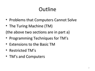
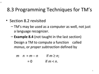
This document discusses programming techniques for Turing machines (TMs), including storing data in states, using multiple tracks, and implementing subroutines. It also covers extensions to basic TMs, such as multitape and nondeterministic TMs. Restricted TMs like those with semi-infinite tapes, stack machines, and counter machines are also examined. Finally, the document informally argues that TMs and modern computers are equally powerful models of computation.

1. Turing Machines (part b)
1
LuxemburgLuxemburg

2. Outline
• Problems that Computers Cannot Solve
• The Turing Machine (TM)
(the above two sections are in part a)
• Programming Techniques for TM’s
• Extensions to the Basic TM
• Restricted TM’s
• TM’s and Computers
2

3. 8.3 Programming Techniques for TM’s
• Concepts to be taught
– Showing how a TM computes.
– Indicating that TM’s are as powerful as
conventional computers.
– Even some extended TM’s can be simulated by
the original TM.
3

4. 8.3 Programming Techniques for TM’s
• Section 8.2 revisited
– TM’s may be used as a computer as well, not just
a language recognizer.
– Example 8.4 (not taught in the last section)
Design a TM to compute a function called
monus, or proper subtraction defined by
m n = m − n if m ≥ n;
= 0 if m < n.
4
_×
_×
_×

5. 8.3 Programming Techniques for TM’s
• Section 8.2 revisited
– Example 8.4 (cont’d)
– Assume input integers m and n are put on the input
tape separated by a 1 as 0m
10n
– The TM is M = ({q0
, q1
, …, q6
}, {0, 1}, {0, 1, B}, δ, q0
, B).
– No final state is needed.
5
_×

6. 8.3 Programming Techniques for TM’s
• Section 8.2 revisited
– Example 8.4 (cont’d)
– M conducts the following computation steps:
1. find its leftmost 0 and replaces it by a blank;
2. move right, and look for a 1;
3. after finding a 1, move right continuously
4. after finding a 0, replace it by a 1;
5. move left until finding a blank, & then move one cell
to the right to get a 0;
6. repeat the above process. 6
_×

7. 8.3 Programming Techniques for TM’s
• Section 8.2 revisited
7
symbol
state 0 1 B
q0
(q1
, B, R) (q5
, B, R) -
q1
(q1
, 0, R) (q2
, 1, R) -
q2
(q3
, 1, L) (q2
, 1, R) (q4
, B, L)
q3
(q3
, 0, L) (q3
, 1, L) (q0
, B, R)
q4
(q4
, 0, L) (q4
, B, L) (q6
, 0, R)
q5
(q5
, B, R) (q5
, B, R) (q6
, B, R)
q6
- - -

8. 8.3 Programming Techniques for TM’s
• Section 8.2 revisited
– q0
0010 ⇒1
Bq1
010 ⇒3
B0q1
10 ⇒4
B01q2
0 ⇒5
B0q3
11 ⇒9
Bq3
011 ⇒8
q3
B011 ⇒10
Bq0
011 ⇒1
BBq1
11 ⇒4
BB1q2
1 ⇒6
BB11q2
B ⇒7
BB1q4
1 ⇒12
BBq4
1B ⇒12
Bq4
BBB ⇒13
B0q6
BB
halt!
– q0
0100 ⇒ Bq1
100 ⇒ B1q2
00 ⇒ Bq3
110 ⇒ q3
B110 ⇒
Bq0
110 ⇒ BBq5
10 ⇒ BBBq5
0 ⇒ BBBBq5
B ⇒ BBBBBq6
halt! 8

9. 8.3 Programming Techniques for TM’s
• 8.3.1 Storage in the State
– Technique:
use the finite control of a TM to hold a finite amount
of data, in addition to the state (which represents a
position in a TM “program”).
– Method:
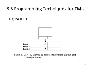
think of the state as [q, A, B, C], for example, when
think of the finite control to hold three data
elements A, B, and C. See the figure in the next page
(Figure 8.13)
9

10. 8.3 Programming Techniques for TM’s
Figure 8.13
10
q
A B C
X
Y
Z
Track 1
Track 2
Track 3
Figure 8.13. A TM viewed as having finite control storage and
multiple tracks.

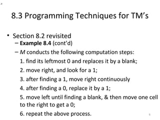
11. 8.3 Programming Techniques for TM’s
• 8.3.1 Storage in the State
– Example 8.6:
Design a TM to recognize 01*
+ 10*.
The set of states
are of the form [qi, X] where qi = q1, q2; X = 0, 1, B.
• The control portion (state) remembers what the
TM is doing (q0 = not read 1st
symbol; q1 = reverse).
• The data portion remembers the first symbol
seen (0, or 1).
11

12. 8.3 Programming Techniques for TM’s
• 8.3.1 Storage in the State
– Example 8.6 (cont’d):
The transition function δ is as follows.
• δ([q0
, B], a) = ([q1
, a], a, R) for a = 0, 1. --- Copying the
symbol it scanned.
• δ([q1
, a],a) = ([q1
, a],a, R) wherea is the complement of
a = 0, 1. --- Skipping symbols which are complements of
the 1st
symbol read (stored in the state as a).
• δ([q1
, a], B) = ([q1
, B], B, R) for a = 0, 1. --- Entering the 12

13. 8.3 Programming Techniques for TM’s
• 8.3.1 Storage in the State
– Example 8.6 (cont’d):
Why does not the TM designed by adding data in
states in the above way increase computing power?
Answer: The states [qi, X] with qi= q1, q2; X = a, b, B, is
just a kind of state labeling, so they can be
transformed, for example, into p1 = [q0, a], p2 = [q0, b],
p3 = [q0, B], …. Then, everything is the same as a
common TM.
13

14. 8.3 Programming Techniques for TM’s
• 8.3.2 Multiple Tracks
– We may think the tape of a TM as composed of
several tracks.
– For example, if there are three tracks, we may use
the tape symbol [X, Y, Z] (like that in Figure 8.13).
– Example 8.7 --- see the textbook. The TM
recognizes the non-CFL language
L = {wcw | w is in (0 + 1)+
}.
– Why does not the power of the TM increase in
this way?
Answer: just a kind of tape symbol labeling.
14

15. 8.3 Programming Techniques for TM’s
• 8.3.3 Subroutines
– The concept of subroutine may also be
implemented for a TM.
– For details, see the textbook.
– Example 8.8 --- design a TM to perform
multiplication on the tape in a way of
transformation as follows:
0m
10n
1 ⇒ 0mn
For details, see the textbook.
15

16. 8.4 Extensions to the Basic TM
• Extended TM’s to be studied:
– Multitape Turing machine
– Nondeterministic Turing machine
• The above extensions make no increase of the
original TM’s power, but make TM’s easier to
use:
– Multitape TM --- useful for simulating real computers
– Nondeterministic TM --- making TM programming
easier.
16

17. 8.4 Extensions to the Basic TM
• 8.4.1 Multitape TM’s
17
Finite
control
Tape 1
Tape 2
Tape 3
Figure 8.16. A multitape TM.

18. 8.4 Extensions to the Basic TM
• 8.4.1 Multitape TM’s
– Initially,
• the input string is placed on the 1st
tape;
• the other tapes hold all blanks;
• the finite control is in its initial state;
• the head of the 1st
tape is at the left end of the input;
• the tape heads of all other tapes are at arbitrary positions.
– A move consists of the following steps:
• the finite control enters a new state;
• on each tape, a symbol is written;
• each tape head moves left or right, or stationary.
18

19. 8.4 Extensions to the Basic TM
• 8.4.2 Equivalence of One –tape & Multitape
TM’s
– Theorem 8.9
Every language accepted by a multitape TM is
recursive enumerable.
(That is, the one-tape TM and the multitape one
are equivalent)
Proof: see the textbook.
19

20. 8.4 Extensions to the Basic TM
• 8.4.3 Running Time and the Many-Tapes-to-
One Construction
– Theorem 8.10
The time taken by the one-tape TM of Theorem
8.9 to simulate n moves of the k-tape TM is O(n2
).
Proof: see the textbook.
– Meaning: the equivalence of the two types of
TM’s is good in the sense that their running times
are roughly the same within polynomial
complexity.
20

21. 8.4 Extensions to the Basic TM
• 8.4.4 Nondeterministic TM’s
– A nondeterministic TM (NTM) has multiple choices of
next moves, i.e.,
δ(q, X) = {(q1
, Y1
, D1
), (q2
, Y2
, D2
), …, (qk
, Yk
, Dk
)}.
– The NTM is not any ‘powerful’ than a deterministic
TM (DTM), as said by the following theorem.
– Theorem 8.11
If MN
is NTM, then there is a DTM MD
such that L(MN
) =
L(MD
). (for proof, see the textbook)
21

22. 8.4 Extensions to the Basic TM
• 8.4.4 Nondeterministic TM’s
– The equivalent DTM constructed for a NTM in the
last theorem may take exponentially more time
than the DTM.
– It is unknown whether or not this exponential
slowdown is necessary!
– More investigation will be done in Chapter 10.
22

23. 8.5 Restricted TM’s
• Restricted TM’s to be studied:
– the tape is infinite only to the right, and the blank
cannot be used as a replacement symbol;
– the tapes are only used as stacks (“stack machines”);
– the stacks are used as counters only (“counter
machines”).
• The above restrictions make no decrease of the
original TM’s power, but are useful for theorem
proving.
• Undecidability of the TM also applies to these
restricted TM’s.
23

24. 8.5 Restricted TM’s
• 8.5.1 TM’s with Semi-infinite Tapes
– Theorem 8.12
Every language accepted by a TM M2
is also
accepted by a TM M1
with the following
restrictions:
• M1
’s head never moves left of its initial position
(so the tape is semi-infinite essential);
• M1
never writes a blank.
(i.e., M1 and M2 are equivalent)
Proof. See the textbook.
24

25. 8.5 Restricted TM’s
• 8.5.2 Multistack Machines
– Multistack machines, which are restricted versions
of TM’s, may be regarded as extensions of
pushdown automata (PDA’s).
– Actually, a PDA with two stacks has the same
computation power as the TM.
– See Fig.8.20 for a figure of a multistack TM.
– Theorem 8.13
If a language is accepted by a TM, then it is accepted
by a two-stack machine.
Proof. See the textbook. 25

26. 8.5 Restricted TM’s
• 8.5.3 Counter Machines
– There are two ways to think of a counter machine.
– Way 1: as a multistack machine with each stack
replaced by a counter regarded to be on a tape of a
TM.
• A counter holds any nonnegative integer.
• The machine can only distinguish zero and
nonzero counters.
• A move conducts the following operations:
–changing the state;
–add or subtract 1 from a counter which cannot
becomes negative. 26

27. 8.5 Restricted TM’s
• 8.5.3 Counter Machines
– Way 2: as a restricted multistack machine with each
stack replaced by a counter implemented on a stack
of a PDA.
• There are only two stack symbols Z0 and X.
• Z0 is the initial stack symbol, like that of a PDA.
• Can replace Z0only by Xi
Z0 for some i ≥ 0.
• Can replace X only by Xi
for some i ≥ 0.
– For an example of a counter machine of the 2nd
type,
do the exercise (part a) of this chapter. 27

28. 8.5 Restricted TM’s
• 8.5.4 The Power of Counter Machines
– Every language accepted by a one-counter machine
is a CFL.
– Every language accepted by a counter machine (of
any number of counters) is recursive enumerable.
– Theorem 8.14
Every recursive enumerable language is accepted by
a three-counter machine.
Proof. See the textbook.
28

29. 8.5 Restricted TM’s
• 8.5.4 The Power of Counter Machines
– Theorem 8.15
Every recursive enumerable language is accepted by
a two-counter machine.
Proof. See the textbook.
29

30. 8.6 Turing Machines and Computers
• In this section, it is shown informally that:
– a computer can simulate a TM; and that
– a TM can simulate a computer.
• That means:
the real computer we use every day is nearly an
implementation of the maximal computational model.
under the assumptions that
– the memory space (including registers, RAM, hard disks,
…) is infinite in size.
– the address space is infinite (not only that defined by 32
bits used in most computers today).
30

31. 8.7 Turing Machines and Computers
• 8.7.1 Simulating a TM by Computer
– If the previous two assumptions are not satisfied,
then a real computer is actually a finite
automaton!
– We can simulate an infinite memory space by
“storage swapping.”
– Also, simulating the infinite tape of the TM by two
stacks of disks, respectively for the left portion
and the right portion of the tape, with the head as
the middle.
31

32. 8.6 Turing Machines and Computers
• 8.6.1 Simulating a TM by a Computer
– Write a program on the computer to simulate the
states and the symbols of the TM in the following
way:
• encode the states as character strings;
• encode the tape symbols with fixed-length character
strings, too;
• use a table of transitions to determine each move.
– By the above way, a TM may be said to be
simulatable by a program of a real computer
(informally)! 32

33. 8.6 Turing Machines and Computers
• 8.6.2 Simulating a Computer by a TM
– Meaning of this section:
The TM is as powerful as a modern-day computer
though it seems so simple!
– Sketch of the simulation using a Multitape TM (see
Fig. 8.22)
• use a TM tape as the computer memory;
• use a TM tape to simulate the instruction counter;
• use a TM tape for the memory address;
• use a TM tape as scratch to perform computation
operations on it. 33

34. 8.6 Turing Machines and Computers
• 8.6.2 Simulating a Computer by a TM
– Meaning of this section: the TM is as powerful as a
modern-day computer though it seems so simple!
– Sketch of using a Multitape TM (see Fig. 8.22) to
simulate the sequence of instructions (described by
an assembly-language program usually) of the
computer:
• use a TM tape as the computer memory;
• use a TM tape to simulate the instruction counter;
• use a TM tape for the memory address;
• use a TM tape as scratch to perform computation
operations on it. 34

35. 8.6 Turing Machines and Computers
• 8.6.2 Simulating a Computer by a TM
– The TM simulates the instruction cycle of the
computer using the above tapes. For more details,
see pp. 366-367 of the textbook.
– Assume that the computer has an “accept”
instruction. The TM simulate it and enters an
accepting state.
– Essence of simulation above:
• the TM has many tapes of different purposes to use;
• the TM can do any computation on the tapes.
35

36. 8.6 Turing Machines and Computers
• 8.6.3 Comparing the Running Times of Computers
and Turing Machines
– If the simulation discussed in the previous section take
exponential times, then it is less meaningful. What is the
fact?
– We hope the two types of machines are polynomially
equivalent, i.e., the computer is simulatable by the TM
in polynomial time. The answer is yes! (cont’d)
36

37. 8.6 Turing Machines and Computers
• 8.6.3 Comparing the Running Times of
Computers and Turing Machines
– Theorem 8.17
If a computer:
(1) has only instructions that increase the
maximum word length by at most 1 and;
(2) has only instructions that a multitape TM can
perform on words of length k in (k2
) steps or less,
then the TM described in Section 8.6.2 can simulate
n steps of the computer in O(n3
) of its own steps.
(see the textbook for a proof)
37

38. 8.6 Turing Machines and Computers
• 8.6.3 Comparing the Running Times of
Computers and Turing Machines
– Theorem 8.18
A computer of the type described in Theorem
8.17 can be simulated for n steps by a one-tape
TM, using at most O(n6
) steps for the TM.
– Conclusion: the TM is as “powerful” as a real
computer seen today!
38

39. Brain Activity
• Which word is the odd one out:
First Second Third Forth Fifth Sixth Seventh
Eighth
• What ends in a 'w' but has no end?
39

40. Brain Activity
• Fourth
• Rainbow
40

41. Brain Activity
• What demands an answer but asks no
question?
• What does this represent?
COF FEE
What is this phrase? XQQQME
41

42. Brain Activity
• Telephone
• Coffee break
• X Q’s ME
42