Time value of money 2

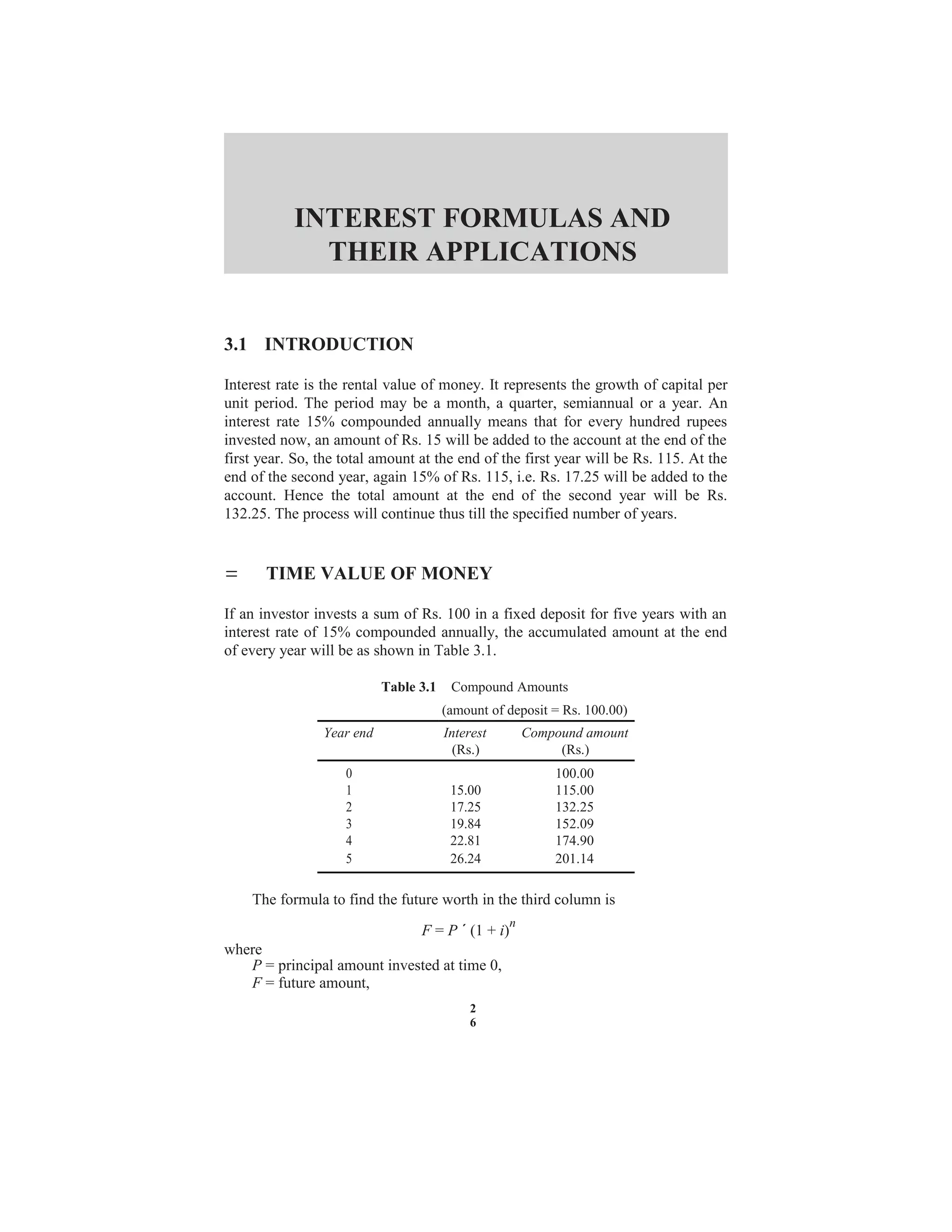
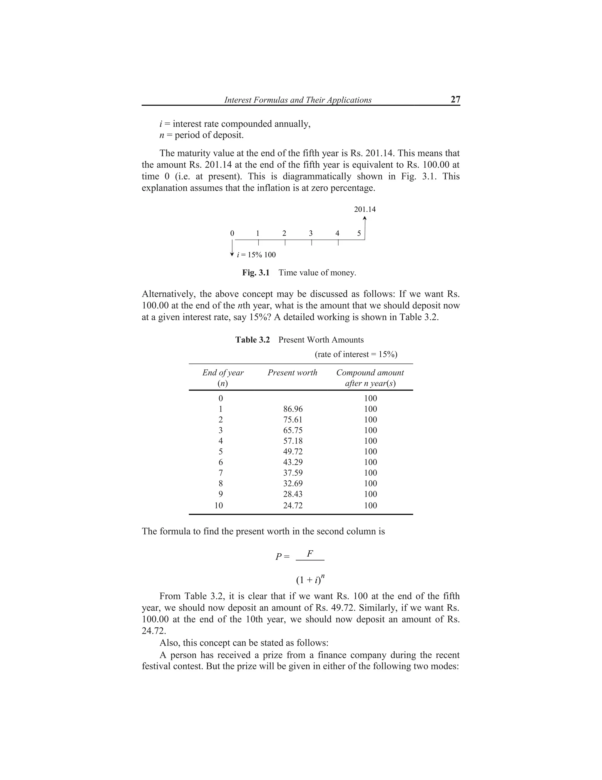
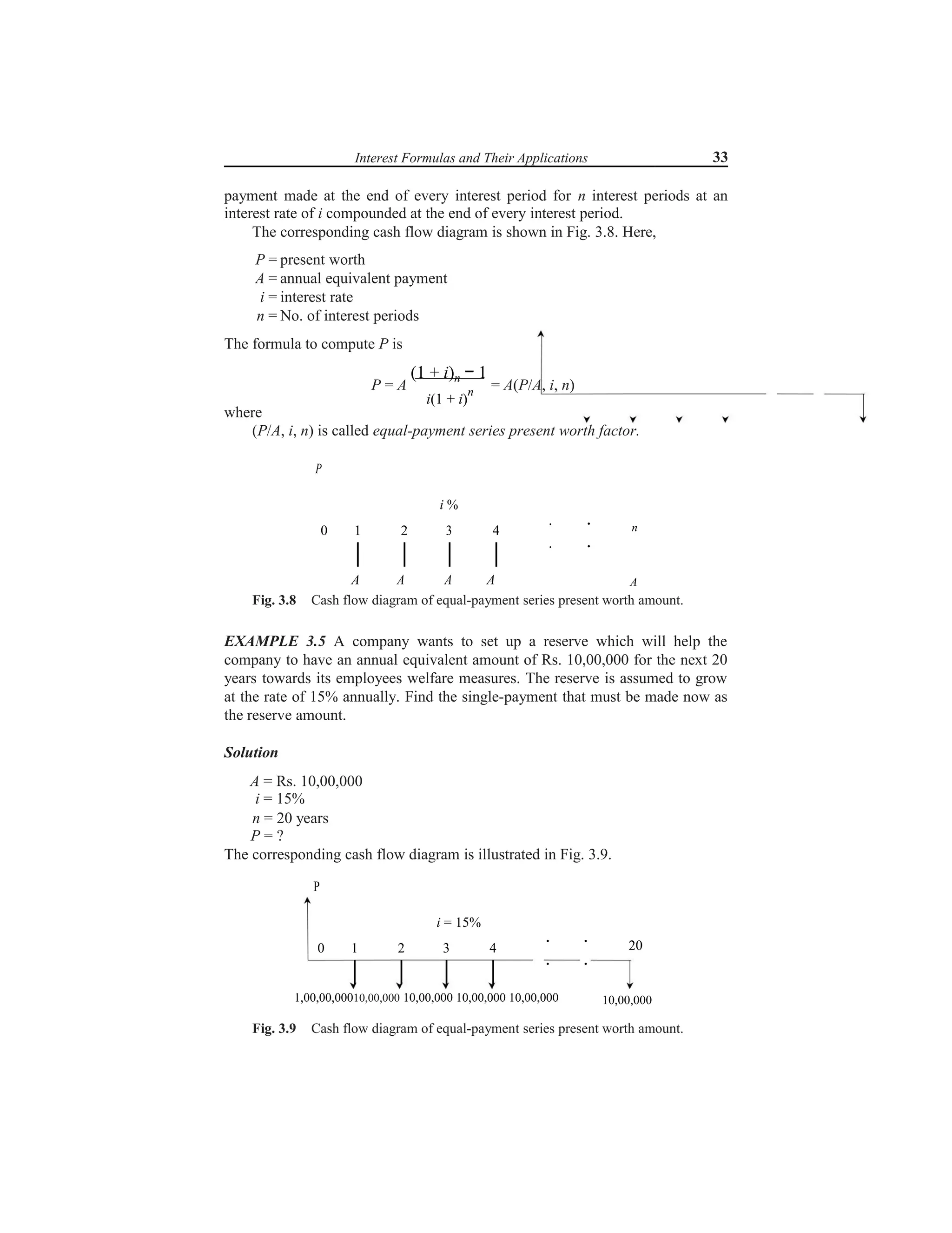
INTEREST FORMULAS AND
THEIR APPLICATIONS
3.1 INTRODUCTION
Interest rate is the rental value of money. It represents the growth of capital per
unit period. The period may be a month, a quarter, semiannual or a year. An
interest rate 15% compounded annually means that for every hundred rupees
invested now, an amount of Rs. 15 will be added to the account at the end of the
first year. So, the total amount at the end of the first year will be Rs. 115. At the
end of the second year, again 15% of Rs. 115, i.e. Rs. 17.25 will be added to the
account. Hence the total amount at the end of the second year will be Rs.
132.25. The process will continue thus till the specified number of years.
= TIME VALUE OF MONEY
If an investor invests a sum of Rs. 100 in a fixed deposit for five years with an
interest rate of 15% compounded annually, the accumulated amount at the end
of every year will be as shown in Table 3.1.
Table 3.1 Compound Amounts
(amount of deposit = Rs. 100.00)
Year end Interest Compound amount
(Rs.) (Rs.)
0 100.00
1 15.00 115.00
2 17.25 132.25
3 19.84 152.09
4 22.81 174.90
5 26.24 201.14
The formula to find the future worth in the third column is
F = P ´ (1 + i)
n
where
P = principal amount invested at time 0,
F = future amount,
2
6

Interest Formulas and Their Applications 27
i = interest rate compounded annually,
n = period of deposit.
The maturity value at the end of the fifth year is Rs. 201.14. This means that
the amount Rs. 201.14 at the end of the fifth year is equivalent to Rs. 100.00 at
time 0 (i.e. at present). This is diagrammatically shown in Fig. 3.1. This
explanation assumes that the inflation is at zero percentage.
201.14
0 1 2 3 4 5
i = 15% 100
Fig. 3.1 Time value of money.
Alternatively, the above concept may be discussed as follows: If we want Rs.
100.00 at the end of the nth year, what is the amount that we should deposit now
at a given interest rate, say 15%? A detailed working is shown in Table 3.2.
Table 3.2 Present Worth Amounts
(rate of interest = 15%)
End of year Present worth Compound amount
(n) after n year(s)
0 100
1 86.96 100
2 75.61 100
3 65.75 100
4 57.18 100
5 49.72 100
6 43.29 100
7 37.59 100
8 32.69 100
9 28.43 100
10 24.72 100
The formula to find the present worth in the second column is
P = F
(1 + i)
n
From Table 3.2, it is clear that if we want Rs. 100 at the end of the fifth
year, we should now deposit an amount of Rs. 49.72. Similarly, if we want Rs.
100.00 at the end of the 10th year, we should now deposit an amount of Rs.
24.72.
Also, this concept can be stated as follows:
A person has received a prize from a finance company during the recent
festival contest. But the prize will be given in either of the following two modes:

28 Engineering Economics
1 Spot payment of Rs. 24.72 or
2 Rs. 100 after 10 years from now (this is based on 15% interest rate
compounded annually).
If the prize winner has no better choice that can yield more than 15%
interest rate compounded annually, and if 15% compounded annually is the
common interest rate paid in all the finance companies, then it makes no
difference whether he receives Rs. 24.72 now or Rs. 100 after 10 years.
On the other hand, let us assume that the prize winner has his own business
wherein he can get a yield of 24% interest rate (more than 15%) compounded
annually, it is better for him to receive the prize money of Rs. 24.72 at present
and utilize it in his business. If this option is followed, the equivalent amount for
Rs. 24.72 at the end of the 10th year is Rs. 212.45. This example clearly
demonstrates the time value of money.
3.3 INTEREST FORMULAS
While making investment decisions, computations will be done in many ways.
To simplify all these computations, it is extremely important to know how to use
interest formulas more effectively. Before discussing the effective application of
the interest formulas for investment-decision making, the various interest
formulas are presented first.
Interest rate can be classified into simple interest rate and compound
interest rate.
In simple interest, the interest is calculated, based on the initial deposit for
every interest period. In this case, calculation of interest on interest is not
applicable. In compound interest, the interest for the current period is computed
based on the amount (principal plus interest up to the end of the previous period)
at the beginning of the current period.
The notations which are used in various interest formulae are as follows:
P = principal amount
n = No. of interest periods
3.4 = interest rate (It may be compounded monthly, quarterly,
semiannually or annually)
F = future amount at the end of year n
A = equal amount deposited at the end of every interest period
G = uniform amount which will be added/subtracted period after period to/
from the amount of deposit A1 at the end of period 1
3.3.1 Single-Payment Compound Amount
Here, the objective is to find the single future sum (F) of the initial payment (P)
made at time 0 after n periods at an interest rate i compounded every period. The
cash flow diagram of this situation is shown in Fig. 3.2.

. .
. .0 1 2 3 4
P i %
F
n
Fig. 3.2 Cash flow diagram of single-payment compound amount.
The formula to obtain the single-payment compound amount is
F = P(1 + i)
n
= P(F/P, i, n)
where
(F/P, i, n) is called as single-payment compound amount factor.
EXAMPLE 3.1 A person deposits a sum of Rs. 20,000 at the interest rate of
18% compounded annually for 10 years. Find the maturity value after 10 years.
Solution
P = Rs. 20,000
i = 18% compounded annually
n = 10 years
1.= P(1 + i)
n
= P(F/P, i, n)
←20,000 (F/P, 18%, 10)
←20,000 ´ 5.234 = Rs. 1,04,680
The maturity value of Rs. 20,000 invested now at 18% compounded yearly
is equal to Rs. 1,04,680 after 10 years.
1. Single-Payment Present Worth Amount
Here, the objective is to find the present worth amount (P) of a single future sum
(F) which will be received after n periods at an interest rate of i compounded at
the end of every interest period.
The corresponding cash flow diagram is shown in Fig. 3.3.
F
. .
. .0 1 2 3 4 n
P i %
Fig. 3.3 Cash flow diagram of single-payment present worth amount.
The formula to obtain the present worth is
F
P =
(1 + i)n
= F(P/F, i, n)
where
(P/F, i, n) is termed as single-payment present worth factor.

EXAMPLE 3.2 A person wishes to have a future sum of Rs. 1,00,000 for his
son’s education after 10 years from now. What is the single-payment that he
should deposit now so that he gets the desired amount after 10 years? The bank
gives 15% interest rate compounded annually.
Solution
F = Rs. 1,00,000
i = 15%, compounded annually
n = 10 years
9. = F/(1 + i)
n
= F(P/F, i, n)
←1,00,000 (P/F, 15%, 10)
← 1,00,000 ´ 0.2472
←Rs. 24,720
The person has to invest Rs. 24,720 now so that he will get a sum of Rs.
1,00,000 after 10 years at 15% interest rate compounded annually.
3.3.3 Equal-Payment Series Compound Amount
In this type of investment mode, the objective is to find the future worth of n
equal payments which are made at the end of every interest period till the end of
the nth interest period at an interest rate of i compounded at the end of each
interest period. The corresponding cash flow diagram is shown in Fig. 3.4.
i %
0 1 2 3 4
A A A A
. .
. .
F
n
A
Fig. 3.4 Cash flow diagram of equal-payment series compound amount.
In Fig. 3.4,
A = equal amount deposited at the end of each interest period
10. = No. of interest
periods i = rate of interest
F = single future amount
The formula to get F is
(1 + i)
n
− 1
F = A = A(F/A, i, n)
i
where
(F/A, i, n) is termed as equal-payment series compound amount factor.
EXAMPLE 3.3 A person who is now 35 years old is planning for his retired life.
He plans to invest an equal sum of Rs. 10,000 at the end of every year for

the next 25 years starting from the end of the next year. The bank gives 20%
interest rate, compounded annually. Find the maturity value of his account when
he is 60 years old.
Solution
A = Rs. 10,000
n = 25 years
i = 20%
F = ?
F
i = 20%
0 1 2 3 4
10,000 10,000 10,000 10,000
. .
. . 25
10,000
Fig. 3.5 Cash flow diagram of equal-payment series compound amount.
F = A (1 + i)
n
− 1
i
15. A(F/A, i, n)
16. 10,000(F/A, 20%, 25)
17. 10,000 ´ 471.981
18. Rs. 47,19,810
The future sum of the annual equal payments after 25 years is equal to Rs.
47,19,810.
3.3.4 Equal-Payment Series Sinking Fund
In this type of investment mode, the objective is to find the equivalent amount
(A) that should be deposited at the end of every interest period for n interest
periods to realize a future sum (F) at the end of the nth interest period at an
interest rate of i.
i %
0 1 2 3 4
A A A A
i %
. .
. .
F
n
A
Fig. 3.6 Cash flow diagram of equal-payment series sinking fund.

In Fig. 3.6,
A = equal amount to be deposited at the end of each interest period n =
No. of interest periods
i = rate of interest
F = single future amount at the end of the nth period
The formula to get F is
i
A = F = F(A/F, i, n) (1 + i)
n
− 1
where
(A/F, i, n) is called as equal-payment series sinking fund factor.
EXAMPLE 3.4 A company has to replace a present facility after 15 years at an
outlay of Rs. 5,00,000. It plans to deposit an equal amount at the end of every
year for the next 15 years at an interest rate of 18% compounded annually. Find
the equivalent amount that must be deposited at the end of every year for the
next 15 years.
Solution
F = Rs. 5,00,000
n = 15 years
i = 18%
A = ?
i = 18%
0 1 2 3 4 . .
. .
5,00,000
15
A A A A A
Fig. 3.7 Cash flow diagram of equal-payment series sinking fund.
i
A = F = F(A/F, i, n) (1 + i)
n
− 1
16. 5,00,000(A/F, 18%, 15)
17. 5,00,000 ´ 0.0164
18. Rs. 8,200
The annual equal amount which must be deposited for 15 years is Rs. 8,200.
4.2 Equal-Payment Series Present Worth Amount
The objective of this mode of investment is to find the present worth of an equal

payment made at the end of every interest period for n interest periods at an
interest rate of i compounded at the end of every interest period.
The corresponding cash flow diagram is shown in Fig. 3.8. Here,
P = present worth
A = annual equivalent payment
i = interest rate
The formula to compute P is
P = A
(1 + i)n − 1
= A(P/A, i, n)
i(1 + i)
n
where
(P/A, i, n) is called equal-payment series present worth factor.
P
i %
0 1 2 3 4
A A A A
. .
. .
n
A
Fig. 3.8 Cash flow diagram of equal-payment series present worth amount.
EXAMPLE 3.5 A company wants to set up a reserve which will help the
company to have an annual equivalent amount of Rs. 10,00,000 for the next 20
years towards its employees welfare measures. The reserve is assumed to grow
at the rate of 15% annually. Find the single-payment that must be made now as
the reserve amount.
Solution
A = Rs. 10,00,000
i = 15%
n = 20 years
P = ?
The corresponding cash flow diagram is illustrated in Fig. 3.9.
P
i = 15%
. .
0 1 2 3 4
. .
1,00,00,00010,00,000 10,00,000 10,00,000 10,00,000
20
10,00,000
Fig. 3.9 Cash flow diagram of equal-payment series present worth amount.

P = A
( 1 + i)
n
− 1
= A(P/A, i, n)
i (1 + i)
n
4.4 10,00,000 ´ (P/A, 15%, 20)
4.5 10,00,000 ´ 6.2593
4.6 Rs. 62,59,300
The amount of reserve which must be set-up now is equal to Rs. 62,59,300.
= Equal-Payment Series Capital Recovery Amount
The objective of this mode of investment is to find the annual equivalent amount
(A) which is to be recovered at the end of every interest period for n interest
periods for a loan (P) which is sanctioned now at an interest rate of i
compounded at the end of every interest period (see Fig. 3.10).
P
i %
0 1 2 3 4
A A A A
. .
. .
n
A
Fig. 3.10 Cash flow diagram of equal-payment series capital recovery amount.
In Fig. 3.10,
P = present worth (loan amount)
A = annual equivalent payment (recovery amount)
i = interest rate
The formula to compute P is as follows:
i(1 + i)
n
A = P = P(A/P, i, n)
(1 + i)
n
− 1
where,
(A/P, i, n) is called equal-payment series capital recovery factor.
EXAMPLE 3.6 A bank gives a loan to a company to purchase an equipment
worth Rs. 10,00,000 at an interest rate of 18% compounded annually. This
amount should be repaid in 15 yearly equal installments. Find the installment
amount that the company has to pay to the bank.
Solution
P = Rs. 10,00,000
i = 18%
n = 15 years
A = ?

10,00,000
i = 18%
0 1 2 3 4
A A A A
. .
. .
15
A
Fig. 3.11 Cash flow diagram of equal-payment series capital recovery amount.
A = P
i(1 + i)
n
= P(A/P, i, n)
(1 + i)
n
− 1
= 10,00,000 ´ (A/P, 18%, 15)
= 10,00,000 ´ (0.1964)
= Rs. 1,96,400
The annual equivalent installment to be paid by the company to the bank is
Rs. 1,96,400.
3.3.7 Uniform Gradient Series Annual Equivalent Amount
The objective of this mode of investment is to find the annual equivalent amount
of a series with an amount A1 at the end of the first year and with an equal
increment (G) at the end of each of the following n – 1 years with an interest
rate i compounded annually.
0 1 2 3 4 . .
. .
1
0
A
1 1+G
A1+2G
A1+3
G
A1+ (n – 1)G
Fig. 3.12 Cash flow diagram of uniform gradient series annual equivalent amount.
The formula to compute A under this situation is
(1 + i)
n
− in − 1
A = A1 + G
i(1 + i)
n
−
i = A1 + G (A/G, i, n)
where
(A/G, i, n) is called uniform gradient series factor.
EXAMPLE 3.7 A person is planning for his retired life. He has 10 more years

of service. He would like to deposit 20% of his salary, which is Rs. 4,000, at the
end of the first year, and thereafter he wishes to deposit the amount with an
annual increase of Rs. 500 for the next 9 years with an interest rate of 15%. Find
the total amount at the end of the 10th year of the above series.
Solution Here,
A1 = Rs. 4,000
G = Rs. 500
i = 15%
n = 10 years
A = ? & F = ?
The cash flow diagram is shown in Fig. 3.13.
i = 15%
0 1 2 3 4
4,000 4,000 + 500
4,000 + 1,000
4,000 + 1,500
. .
. .
10
4,000 + 4,500
(1 + i)
n
− in − 1
A = A1 + G
i(1 + i)
n
− i
=A1 + G(A/G, i, n)
= 4,000 + 500(A/G, 15%, 10)
= 4,000 + 500 ´ 3.3832
= Rs. 5,691.60
This is equivalent to paying an equivalent amount of Rs. 5,691.60 at the end of
every year for the next 10 years. The future worth sum of this revised series at
the end of the 10th year is obtained as follows:
== A(F/A, i, n)
←A(F/A, 15%, 10)
← 5,691.60(20.304)
← Rs. 1,15,562.25
At the end of the 10th year, the compound amount of all his payments will
be Rs. 1,15,562.25.
EXAMPLE 3.8 A person is planning for his retired life. He has 10 more years of
service. He would like to deposit Rs. 8,500 at the end of the first year and

thereafter he wishes to deposit the amount with an annual decrease of Rs. 500
for the next 9 years with an interest rate of 15%. Find the total amount at the end
of the 10th year of the above series.
Solution Here,
A1 =Rs. 8,500
G =–Rs. 500
i =15%
n =10 years
A =? & F = ?
The cash flow diagram is shown in Fig. 3.14.
i = 15%
0 1 2 3 4
7,000
7,500
8,000
8,500
. .
. .
10
4,000
A = A1 – G (1 + i)
n
− in − 1
i(1 + i)
n
− i
=A1 – G (A/G, i, n)
=8,500 – 500(A/G, 15%, 10)
= 8,500 – 500 ´ 3.3832
= Rs. 6,808.40
This is equivalent to paying an equivalent amount of Rs. 6,808.40 at the end of
every year for the next 10 years.
The future worth sum of this revised series at the end of the 10th year is
obtained as follows:
== A(F/A, i, n)
←A(F/A, 15%, 10)
← 6,808.40(20.304)
← Rs. 1,38,237.75
At the end of the 10th year, the compound amount of all his payments is Rs.
1,38,237.75.
= Effective Interest Rate
Let i be the nominal interest rate compounded annually. But, in practice, the
compounding may occur less than a year. For example, compounding may be
monthly, quarterly, or semi-annually. Compounding monthly means that the
interest is computed at the end of every month. There are 12 interest periods in

a year if the interest is compounded monthly. Under such situations, the formula
to compute the effective interest rate, which is compounded annually, is
Effective interest rate, R = E1+ i/CJC
− 1
where,
i = the nominal interest rate
C = the number of interest periods in a year.
EXAMPLE 3.9 A person invests a sum of Rs. 5,000 in a bank at a nominal
interest rate of 12% for 10 years. The compounding is quarterly. Find the
maturity amount of the deposit after 10 years.
Solution
P = Rs. 5,000
n = 10 years
i = 12% (Nominal interest rate)
F = ?
METHOD 1
No. of interest periods per year = 4
No. of interest periods in 10 years = 10 ´ 4 = 40
Revised No. of periods (No. of quarters), N = 40
Interest rate per quarter, r = 12%/4
= 3%, compounded quarterly.
= = P(1 + r)
N
= 5,000(1 + 0.03)
40
= Rs. 16,310.19
METHOD 2
No. of interest periods per year, C = 4
Effective interest rate, R = (1 + i/C )
C
– 1
1.(1 + 12%/4)
4
– 1
2. 12.55%, compounded annually.
← = P(1 + R)
n
= 5,000(1 + 0.1255)
10
= Rs. 16,308.91
= BASES FOR COMPARISON OF ALTERNATIVES
In most of the practical decision environments, executives will be forced to
select the best alternative from a set of competing alternatives. Let us assume
that an organization has a huge sum of money for potential investment and there
are three different projects whose initial outlay and annual revenues during their
lives are known. The executive has to select the best alternative among these
three competing projects.

There are several bases for comparing the worthiness of the projects. These
bases are:
= Present worth method
= Future worth method
= Annual equivalent method
= Rate of return method
These methods are discussed in detail in Chapters 4–7.
QUESTIONS
= Explain the time value of money.
= Give practical applications of various interest formulas.
= A person deposits a sum of Rs. 1,00,000 in a bank for his son’s education
who will be admitted to a professional course after 6 years. The bank pays
15% interest rate, compounded annually. Find the future amount of the
deposited money at the time of admitting his son in the professional course.
= A person needs a sum of Rs. 2,00,000 for his daughter’s marriage which
will take place 15 years from now. Find the amount of money that he should
deposit now in a bank if the bank gives 18% interest, compounded annually.
= A person who is just 30 years old is planning for his retired life. He plans to
invest an equal sum of Rs. 10,000 at the end of every year for the next 30
years starting from the end of next year. The bank gives 15% interest rate,
compounded annually. Find the maturity value of his account when he is 60
years old.
= A company is planning to expand its business after 5 years from now. The
expected money required for the expansion programme is Rs. 5,00,00,000.
The company can invest Rs. 50,00,000 at the end of every year for the next
five years. If the assured rate of return of investment is 18% for the
company, check whether the accumulated sum in the account would be
sufficient to meet the fund for the expansion programme. If not, find the
difference in amounts for which the company should make some other
arrangement after 5 years.
= A financial institution introduces a plan to pay a sum of Rs. 15,00,000 after 10
years at the rate of 18%, compounded annually. Find the annual equivalent
amount that a person should invest at the end of every year for the next 10 years
to receive Rs. 15,00,000 after 10 years from the institution.
= A company is planning to expand its business after 5 years from now. The
money required for the expansion programme is Rs. 4,00,00,000. What
annual equivalent amount should the company deposit at the end of every
year at an interest rate of 15% compounded annually to get Rs. 4,00,00,000
after 5 years from now?

= A company wants to set-up a reserve which will help it to have an annual
equivalent amount of Rs. 15,00,000 for the next 20 years towards its
employees welfare measures. The reserve is assumed to grow at the rate of
15% annually. Find the single-payment that must be made as the reserve
amount now.
= An automobile company recently advertised its car for a down payment of
Rs. 1,50,000. Alternatively, the car can be taken home by customers
without making any payment, but they have to pay an equal yearly amount
of Rs. 25,000 for 15 years at an interest rate of 18%, compounded annually.
Suggest the best alternative to the customers.
= A company takes a loan of Rs. 20,00,000 to modernize its boiler section.
The loan is to be repaid in 20 equal installments at 12% interest rate,
compounded annually. Find the equal installment amount that should be
paid for the next 20 years.
= A bank gives loan to a company to purchase an equipment which is worth
of Rs. 5,00,000, at an interest rate of 18% compounded annually. This
amount should be repaid in 25 yearly equal installments. Find the
installment amount that the company has to pay to the bank.
= A working woman is planning for her retired life. She has 20 more years of
service. She would like to deposit 10% of her salary which is Rs. 5,000 at
the end of the first year and thereafter she wishes to deposit the same
amount (Rs. 5,000) with an annual increase of Rs. 1,000 for the next 14
years with an interest rate of 18%. Find the total amount at the end of the
15th year of the above series.
= Consider the following cash flow diagram. Find the total amount at the end
of the 10th year at an interest rate of 12%, compounded annually.
i = 15%
0 1 2 3 4
8,000
8,000 + 1,000
8,000 + 2,000
8,000 + 3,000
. . 10
. .
8,000 + 9,000
1. A person is planning for his retired life. He has 10 more years of service. He
would like to deposit 20% of his salary, which is Rs. 10,000, at the end of
the first year and thereafter he wishes to deposit the same amount (Rs.
10,000) with an annual increase of Rs. 2,000 for the next 9 years with an
interest rate of 20%. Find the total amount at the end of the 10th year of the
above series.

4. A person is planning for his retired life. He has 10 more years of service. He
would like to deposit Rs. 30,000 at the end of the first year and thereafter he
wishes to deposit the same amount (Rs. 30,000) with an annual decrease of
Rs. 2,000 for the next 9 years with an interest rate of 18%. Find the total
amount at the end of the 10th year of the above series.
5. A person invests a sum of Rs. 50,000 in a bank at a nominal interest rate of
18% for 15 years. The compounding is monthly. Find the maturity amount
of the deposit after 15 years.

11
INFLATION ADJUSTED DECISIONS
INTRODUCTION
A general inflationary trend in the cost of goods is common everywhere due to
various interacting factors. If the rate of inflation is very high, it will produce
extremely serious consequences for both individuals and institutions.
Inflation is the rate of increase in the prices of goods per period. So, it has a
compounding effect. Thus, prices that are inflated at a rate of 7% per year will
increase 7% in the first year, and for the next year the expected increase will be 7%
of these new prices. The same is true for succeeding years and hence the rate of
inflation is compounded in the same manner that an interest rate is compounded. If
the average inflation over six years period is 7%, then the prices at the beginning of
the seventh year would be 150% that of the first year by assuming 100% for the
prices at the beginning of the first year of the six-year period.
If economic decisions are taken without considering the effect of inflation
into account, most of them would become meaningless and as a result the
organizations would end up with unpredictable return.
But there is always difficulty in determining the rate of inflation. The
world-wide trend/wish is to curtail inflation. But due to various reasons, it is
very difficult to have zero inflation. For practical decision making, an average
estimate may be assumed depending on the period of the proposals under
consideration. Hence, we need a procedure which will combine the effects of
inflation rate and interest rate to take realistic economic decision.
PROCEDURE TO ADJUST INFLATION
A procedure to deal with this situation is summarized now.
Estimate all the costs/returns associated with an investment proposal in
terms of today’s rupees.
Modify the costs/returns estimated in step 1 using an assumed inflation rate
so that at each future date they represent the costs/returns at that date in
terms of the rupees that must be expended/received at that time,
respectively.
As per our requirement, calculate either the annual equivalent amount or
future amount or present amount of the cash flow resulting from step 2
by considering the time value of money.
14
7

EXAMPLE 11.1 Suppose a 40-year old man is planning for his retirement. He
plans to retire at the age of 60 and estimates that he can live comfortably on Rs.
24,000 per year in terms of today’s rupee value. He can invest his savings at
15% compounded annually. Assume an average inflation rate of 9% for the next
30 years.
What equal amount should he save each year until he retires so that he can
make withdrawals at the end of each year commencing from the end of the 21st
year from now that will allow him to live as comfortably as he desires for 10
years beyond his retirement?
Solution
Step 1. The estimated future requirement per year in terms of today’s rupees
from his age 61 through 70 is Rs. 24,000.
Step 2. Modification of the costs estimated in step 1 is summarized in Table
11.1. The formula which is given below is used to get future equivalent of Rs.
24,000 with the inflation of 9% per year (IR-inflation rate).
F = P (1 + IR)
n
Table 11.1 Inflated Future Requirements
End of Age Inflated value of Rs. 24,000 at each year end
year (years)
21 61 24,000 ´ (1 + 0.09)
21
= Rs. 1,46,611
22 62 24,000 ´ (1 + 0.09)
22
= Rs. 1,59,806
23 63 24,000 ´ (1 + 0.09)
23
= Rs. 1,74,189
24 64 24,000 ´ (1 + 0.09)
24
= Rs. 1,89,866
25 65 24,000 ´ (1 + 0.09)
25
= Rs. 2,06,954
26 66 24,000 ´ (1 + 0.09)
26
= Rs. 2,25,580
27 67 24,000 ´ (1 + 0.09)
27
= Rs. 2,45,882
28 68 24,000 ´ (1 + 0.09)
28
= Rs. 2,68,011
29 69 24,000 ´ (1 + 0.09)
29
= Rs. 2,92,132
30 70 24,000 ´ (1 + 0.09)
30
= Rs. 3,18,424
Step 3. Now, the calculation of the equivalent amount of cash flow as per
the requirement is presented.
The overall cash flow diagram for the savings and withdrawal in terms of
future rupees is shown in Fig. 11.1.
3,18,424
2,92,132
1,59,806
1,46,611
0 1 2 3 . . 19 20 . .
21 22 29 30
A A A A A
Fig. 11.1 Overall cash flow diagram.

Inflation Adjusted Decisions 149
The sum of the present equivalents of the year end withdrawals from the
year 21 to 30 is computed by assuming the end of the year 20 as the base (time
zero) and it is shown at the end of the year 20 in Fig. 11.2. The method of
computing the present equivalent of the withdrawals is as follows:
PW(i = 15%) = 1,46,611/(1 + 0.15)
1
+ 1,59,806/(1 + 0.15)
2
0 1,74,189/(1 + 0.15)
3
+ 1,89,866/(1 + 0.15)
4
1 2,06,954/(1 + 0.15)
5
+ 2,25,580/(1 + 0.15)
6
2 2,45,882/(1 + 0.15)
7
+ 2,68,011/(1 + 0.15)
8
3 2,92,132/(1 + 0.15)
9
+ 3,18,424/(1 + 0.15)
10
Rs. 10,13,631.
10,13,631(F)
0 1 2 3 19 20
A A A A A
Fig. 11.2 Equivalent cash flow diagram.
The annual equivalent amount (A), which should be invested from the end of
year 1 (age 41) to year 20 (age 60), is computed using the following formula.
= F(A/F, 15%, 20)
0 10,13,631 ´ (0.0098)
1 Rs. 9,934
Recommendation: The person has to invest an amount of Rs. 9,934 at the end
of every year starting from his age 41 (year 1) through 60 (year 20) which will
enable him to make withdrawals at the end of every year starting from his age
61 (year 21) through 70 (year 30) as shown in the Table 11.1 (also in Fig. 11.1).
INFLATION ADJUSTED ECONOMIC LIFE OF MACHINE
(Panneerselvam, 1998)
In any industrial/service organization, equipment/machinery forms an important
element. The productivity of any organization is a function of many factors. It is
largely affected by efficient and effective use of machinery and equipment. So,
operations and maintenance of these equipment are very important to the
organization.
A machine which is purchased today cannot be used forever. It has a
definite economic lifetime. After the economic life, the machine should be
replaced with a substitute machine with similar operational capabilities. This
kind of analysis is called replacement analysis.

The elements of costs involved in the replacement analysis are as follows:
Purchase cost (initial cost)
Annual operation and maintenance cost
Salvage value at the end of every year, if it is significant
The trade-off between different cost elements is shown in Fig. 11.3.
Total cost
Costs
Capital recovery
cost with return
Average operating &
maintenance cost
Economic life
Life of the machine
Fig. 11.3 Chart showing economic life.
From Fig. 11.3, it is clear that the sum of operation and maintenance cost
increases with the life of the machine. But the capital recovery with return
decreases with the life of the machine. The total cost of the machine goes on
decreasing initially but it starts increasing after some years. The year with the
minimum total cost is called as the economic life of the machine.
Limitation of Existing Model
In the case where the machine is replaced due to wear and tear, the following
costs are considered (refer Chapter 8):
Initial cost
Operation and maintenance cost
Salvage value

In the existing model to deal with this type of replacement analysis, the
different cost elements are estimated without taking the effect of inflation into
account.
The annual cost of operation and maintenance of the machine will increase
with the age of the machine due to decline in efficiency of the machine. In the
existing model, this increase in the operation and maintenance cost is taken into
account. But the increase in the operation and maintenance cost due to inflation
is not considered. Similarly, in the existing model, the salvage value is estimated
without taking into account the effect of inflation.
To highlight this particular fact on salvage value, an example is now given. The
internal combustion engines (R.A. Lister) which were made in England during
pre-independence of India are still functioning well. Their resale value is going
up year after year. This may be partly due to inflation and partly due to good
quality of the engine parts. So, consideration of the effect of the inflation
on the economic life of the machine is a realistic approach.
In replacement analysis, a discount rate is usually assumed to reflect the
time value of money. First the concept of replacement analysis is demonstrated
without taking the inflation into account. Then, the same is demonstrated by
taking the effect of inflation into account. At the end, a comparison between the
two models is presented.
Economic Life Determination without Inflationary Effect
The determination of economic life of a machine without considering the effect
of inflation is demonstrated using the following example.
EXAMPLE 11.2 A machine costs Rs. 5,00,000. Its annual operation cost during
the first year is Rs. 40,000 and it increases by Rs. 5,000 every year thereafter.
The maintenance cost during the first year is Rs. 60,000 and it increases by Rs.
6,000 every year thereafter. The resale value of the machine is Rs. 4,00,000 at
the end of the first year and it decreases by Rs. 50,000 every year thereafter.
Assume an interest rate (discounting factor) of 20%.
The method of finding the economic life of the machine with a discounting
factor of 20% at zero inflation rate is summarized in Table 11.2. From the table
it is clear that the total annual equivalent cost is minimum if the machine is used
for 14 years. Hence, the economic life of the machine is 14 years.
Economic Life Determination with Inflationary Effect
The illustration in Section 11.3.2 is reconsidered for analyzing the effect of
inflation on the economic life of the machine. An average annual inflation rate
of 6% is assumed for discussion. The corresponding steps are explained in Table
11.3.
From the Table 11.3, it is clear that the total annual equivalent cost is
minimum if the machine is used for three years. Thus, the economic life of the
machine is three years.

Table 11.2 Determination of Economic Life of the Machine without Inflation
End of Opera- Mainte- Opera- P/F, i, n Present Cumulative Salvage Present Total A/P, i, n Annual
year tion nance tion & worth of of column value worth of present equivalent
cost cost maint. column 4 (6) (S) salvage worth amount
cost
(4) ´ (5)
value
(n) (2) + (3) (8) ´ (5) 5,00,000 +
(10) ´ (11)(i = 20%) Column 7 – 9 (i = 20%)
(1) (2) (3) (4) (5) (6) (7) (8) (9) (10) (11) (12)
(Rs.) (Rs.) (Rs.) (Rs.) (Rs.) (Rs.) (Rs.) (Rs.) (Rs.)
1 40,000 60,000 1,00,000 0.8333 83,330.00 83,330.00 4,00,000 3,33,320.00 2,50,010.00 1.2000 3,00,012.00
2 45,000 66,000 1,11,000 0.6945 77,089.50 1,60,419.50 3,50,000 2,43,075.00 4,17,344.50 0.6546 2,73,193.70
3 50,000 72,000 1,22,000 0.5787 70,601.40 2,31,020.90 3,00,000 1,73,610.00 5,57,410.90 0.4747 2,64,602.90
4 55,000 78,000 1,33,000 0.4823 64,145.90 2,95,166.80 2,50,000 1,20,575.00 6,74,591.80 0.3863 2,60,594.80
5 60,000 84,000 1,44,000 0.4019 57,873.60 3,53,040.40 2,00,000 80,380.00 7,72,660.40 0.3344 2,58,377.60
6 65,000 90,000 1,55,000 0.3349 51,909.50 4,04,949.90 1,50,000 50,235.00 8,54,714.90 0.3007 2,57,012.70
7 70,000 96,000 1,66,000 0.2791 46,330.60 4,51,280.50 1,00,000 27,910.00 9,23,370.50 0.2774 2,56,142.90
8 75,000 1,02,000 1,77,000 0.2326 41,170.20 4,92,450.70 50,000 11,630.00 9,80,820.70 0.2606 2,55,601.80
9 80,000 1,08,000 1,88,000 0.l938 36,434.40 5,28,885.10 0 0.00 10,28,885.00 0.2481 2,55,266.30
10 85,000 1,14,000 1,99,000 0.1615 32,138.50 5,61,023.60 0 0.00 10,61,023.00 0.2385 2,53,054.10
11 90,000 1,20,000 2,10,000 0.1346 28,266.00 5,89,289.60 0 0.00 10,89,289.00 0.2311 2,51,734.80
12 95,000 1,26,000 2,21,000 0.1122 24,796.20 6,14,085.80 0 0.00 11,14,085.00 0.2253 2,51,003.50
13 1,00,000 1,32,000 2,32,000 0.0935 21,692.00 6,35,777.80 0 0.00 11,35,777.00 0.2206 2,50,552.50
14 1,05,000 1,38,000 2,43,000 0.0779 18,929.70 6,54,707.50 0 0.00 11,54,707.00 0.2169 2,50,456.00***
15 1,10,000 1,44,000 2,54,000 0.0649 16,484.60 6,71,192.10 0 0.00 11,71,192.00 0.2139 2,50,517.90
***Total annual equivalent cost is minimum if the machine is used for 14 years.
15
2
EngineeringEconomics

Table 11.3 Determination of Economic Life of the Machine with Inflationary Effect
End of Opera- Mainte- Sum of F/P, i, n Inflated P/F, i, n Present Cumulative Salvage Inflated Present Total A/P, i, n Annual
year tion nance operation operation worth of of column value salvage worth of present (i =20%) equivalent
cost cost & mainte- (i = 6%) & maint. ( i = 20%) column 6 (8) (S) value column 11 worth amount of total
nance cost cost present worth
(n) (2) + (3) (4) ´ (5) (6) ´ (7) (10) ´ (5) (11) ´ (7) 5,00,000 + (13) ´ (14)
(1) (2) (3) (4) (5) (6) (7) (8) (9) (10) (11) (12) Column 9 – 12 (14) (15)
(13)
(Rs.) (Rs.) (Rs.) (Rs.) (Rs.) (Rs.) (Rs.) (Rs.) (Rs.) (Rs.) (Rs.)
1 40,000 60,000 1,00,000 1.060 1,06,000 0.8333 88,329.80 88,329.80 4,00,000 4,24,000 3,53,319.20 2,35,010.6 1.2000 2,82,012.70
2 45,000 66,000 1,11,000 1.124 1,24,764 0.6945 86,648.59 1,74,978.30 3,50,000 3,93,400 2,73,216.30 4,01,762.0 0.6546 2,62,993.40
3 50,000 72,000 1,22,000 1.191 1,45,302 0.5787 84,086.26 2,59,064.60 3,00,000 3,57,300 2,06,769.50 5,52,295.1 0.4747 2,62,174.50 ***
4 55,000 78,000 1,33,000 1.262 1,67,846 0.4823 80,952.12 3,40,016.70 2,50,000 3,15,500 1,52,165.60 6,87,851.1 0.3863 2,65,716.80
5 60,000 84,000 1,44,000 1.338 1,92,672 0.4019 77,434.87 4,17,451.60 2,00,000 2,67,600 1,07,548.40 8,09,903.2 0.3344 2,70,831.60
6 65,000 90,000 1,55,000 1.419 2,19,945 0.3349 73,659.58 4,91,111.20 1,50,000 2,12,850 71,283.46 9,19,827.7 0.3007 2,76,592.20
7 70,000 96,000 1,66,000 1.504 2,49,664 0.2791 69,681.22 5,60,792.40 1,00,000 1,50,400 41,976.64 10,18,815.0 0.2774 2,82,619.50
8 75,000 1,02,000 1,77,000 1.594 2,82,138 0.2326 65,625.29 6,26,417.70 50,000 79,700 18,538.22 11,07,879.0 0.2606 2,88,713.40
9 80,000 1,08,000 1,88,000 1.689 3,17,532 0.l938 61,537.70 6,87,955.40 0 0 0.00 11,87,955.0 0.2481 2,94,731.70
10 85,000 1,14,000 1,99,000 1.791 3,56,409 0.1615 57,560.05 7,45,515.50 0 0 0.00 12,45,515.0 0.2385 2,97,055.40
***Total annual equivalent cost is minimum if machine is used for three years.
InflationAdjustedDecisions15
3

Comparison of results
The results of the two approaches are summarized in Table 11.4 . From the
table, it is clear that the inflation has an effect on the economic life of the
machine. Since it is meaningful and realistic to analyze this type of problem by
considering the effect of inflation, the second approach should be used for such
analysis.
Table 11.4 Results of the Two Approaches
Approach Minimum annual Corresponding
equivalent cost life
(Rs.) (years)
Replacement analysis without
inflation effect 2,50,456.00 14
Replacement analysis with
inflation effect 2,62,174.50 3
EXAMPLE 11.3 A company has received quotes for its recent advertisement for
the purchase of a sophisticated milling machine. The data are as per the estimate
in today’s rupee value.
Machine X Machine Y
Purchase price (Rs.) 15,00,000 20,00,000
Machine life (years) 7 7
Salvage value at the end of
machine life (Rs.) 2,00,000 3,00,000
Annual operating &
maintenance cost (Rs.) 3,00,000 2,50,000
Assuming an average annual inflation of 5% for the next five years,
determine the best machine based on the present worth method. Interest rate is
15%, compounded annually.
Solution
Average annual inflation rate = 5%
Interest rate = 15% compounded annually
Machine X
Purchase price = Rs.15,00,000
Machine life = 7 years
Salvage value at the end of machine life = Rs. 2,00,000
Annual operating & maintenance cost = Rs. 3,00,000
The computation of the present worth of the annual operating and
maintenance costs of the machine X is summarized in Table 11.5.

Table 11.5 Computation of the Present Worth of the Annual Operating and Maintenance
Costs of Machine X
End of Annual operating Inflation Inflated annual P/F, 15%, n Present worth of
year & maintenance factor operating & inflated annual
(n) cost (F/P, maintenance cost operating &
(Rs.) 5%, n) (Rs.) maintenance cost
A B C D E F (Rs.)
B ´ C D ´ E
1 3,00,000 1.050 3,15,000 0.8696 2,73,924
2 3,00,000 1.102 3,30,600 0.7561 2,49,967
3 3,00,000 1.158 3,47,400 0.6575 2,28,416
4 3,00,000 1.216 3,64,800 0.5718 2,08,593
5 3,00,000 1.276 3,82,800 0.4972 1,90,328
6 3,00,000 1.340 4,02,000 0.4323 1,73,785
7 3,00,000 1.407 4,22,100 0.3759 1,58,667
Rs. 14,83,680
The equation for the present worth of the machine X is
PWX(15%) = Purchase price
+ Present worth of inflated annual and operating cost
– Present worth of the salvage value
15,00,000 + 14,83,680 – 2,00,000 ´ (inflation factor) ´
(P/F, 15%, 7)
15,00,000 + 14,83,680 – 2,00,000(F/P, 5%, 7) (P/F, 15%, 7)
15,00,000 + 14,83,680 – 2,00,000 ´ 1.407 ´ 0.3759
Rs. 28,77,901.74
Machine Y
Purchase price = Rs. 20,00,000
Machine life = 7 years
Salvage value at the end of machine life = Rs. 3,00,000
Annual operating & maintenance cost = Rs. 2,50,000
The computation of the present worth of the annual operating and
maintenance costs of the machine Y is summarized in Table 11.6.
Table 11.6 Computation of the Present Worth of the Annual Operating and
Maintenance Costs of Machine Y
End of Annual operating Inflation Inflated annual P/F, 15%, n Present worth of
year & maintenance factor operating & inflated annual
(n) cost (F/P, 5%, n) maintenance cost operating &
(Rs.) (Rs.) maintenance cost
A B C D E F (Rs.)
B ´ C D ´ E
1 2,50,000 1.050 2,62,500 0.8696 2,28,270
2 2,50,000 1.102 2,75,500 0.7561 2,08,306
3 2,50,000 1.158 2,89,500 0.6575 1,90,346
4 2,50,000 1.216 3,04,000 0.5718 1,73,827
5 2,50,000 1.276 3,19,000 0.4972 1,58,607
6 2,50,000 1.340 3,35,000 0.4323 1,44,821
7 2,50,000 1.407 3,51,750 0.3759 1,32,223
Rs. 12,36,400

The expression for the present worth of machine Y is
PWY(15%) = Purchase price
+ present worth of inflated annual and operating cost
– present worth of the salvage value
20,00,000 + 12,36,400 – 3,00,000 ´
(inflation factor) ´ (P/F, 15%, 7)
20,00,000 + 12,36,400 – 3,00,000 (F/P, 5%, 7) (P/F, 15%, 7)
20,00,000 + 12,36,400 – 3,00,000 ´ 1.407 ´ 0.3759
Rs. 30,77,732.61
Remark. Since the present worth cost of machine X is less than that of machine
Y, select machine X.
EXAMPLE 11.4 A company is planning to start an employee welfare fund. It
needs Rs. 50,00,000 during the first year and it increases by Rs. 5,00,000 every
year thereafter up to the end of the 5th year. The above figures are in terms of
todays rupee value. The annual average rate of inflation is 6% for the next five
years. The interest rate is 18%, compounded annually. Find the single deposit
which will provide the required series of fund towards employees welfare
scheme after taking the inflation rate into account.
Solution
Fund requirement during the first year = Rs. 50,00,000
Annual increase in the fund requirement = Rs. 5,00,000
Annual inflation rate = 6%
Interest rate = 18%, compounded annually
The computation of the present worth of the annual fund requirements is
summarized in Table 11.7.
Table 11.7 Computation of the Present Worth of the Annual Requirements
End of Annual fund Inflation Inflated annual P/F, Present worth of
year requirements factor fund requirements 18%, n inflated annual
(n) (Rs.) (F/P, 6%, n) (Rs.) fund requirements
A B C D E F (Rs.)
B ´ C D ´ E
1 50,00,000 1.060 53,00,000 0.8475 44,91,750
2 55,00,000 1.124 61,82,000 0.7182 44,39,912
3 60,00,000 1.191 71,46,000 0.6086 43,49,056
4 65,00,000 1.262 82,03,000 0.5158 42,31,107
5 70,00,000 1.338 93,66,000 0.4371 40,93,879
Rs. 2,16,05,704
The value of the single deposit to be made now to receive the specified series for
the next five years is Rs. 2,16,05,704.

QUESTIONS
Define inflation.
Discuss the impact of inflation on investment decision.
Suppose a 50-year old man is planning for his retirement. He plans to retire at
the age of 60 and estimates that he can live comfortably on Rs. 40,000 per
year in terms of today’s rupee value. Let us assume the average inflation
rate for the next 20 years is 7% per year. This is only an assumption. He can
invest his savings at 20%, compounded annually.
What equal amount should he save each year until he retires so that he
can make withdrawals that will allow him to live as comfortably as he
desires for 10 years beyond his retirement?
A machine costs Rs. 7,00,000. Its annual operation cost during the first year is
Rs. 60,000 and it increases by Rs. 7,000 every year thereafter. The
maintenance cost during the first year is Rs. 80,000 and it increases by Rs.
10,000 every year thereafter. The resale value of the machine is Rs.
3,00,000 at the end of the first year and it decreases by Rs. 75,000 every
year thereafter. Assume an interest rate (discounting factor) of 20% and
inflation of 5%, compounded yearly. Find the inflation adjusted economic
life of the machine.
21
3

APPENDIX—INTEREST TABLES
Interest Table for Annual Compounding with i = 0.25%
n F/p, i, n P/F, i, n F/A, i, n A/F, i, n P/A, i, n A/P, i, n A/G, i, n
1 1.003 0.9975 1.000 1.0000 0.9975 1.0025 0.0000
2 1.005 0.9950 2.003 0.4994 1.9926 0.5019 0.5048
3 1.008 0.9925 3.008 0.3325 2.9851 0.3350 1.0020
4 1.010 0.9901 4.015 0.2491 3.9752 0.2516 1.5012
5 1.013 0.9876 5.025 0.1990 4.9628 0.2015 1.9965
6 1.015 0.9851 6.038 0.1656 5.9479 0.1681 2.4988
7 1.018 0.9827 7.053 0.1418 6.9306 0.1443 2.9938
8 1.020 0.9802 8.070 0.1239 7.9108 0.1264 3.4907
9 1.023 0.9778 9.091 0.1100 8.8886 0.1125 3.9865
10 1.025 0.9753 10.113 0.0989 9.8639 0.1014 4.4830
11 1.028 0.9729 11.139 0.0898 10.8369 0.0923 4.9779
12 1.030 0.9705 12.167 0.0822 11.8074 0.0847 5.4744
13 1.033 0.9681 13.197 0.0758 12.7754 0.0783 5.9676
14 1.036 0.9656 14.230 0.0703 13.7411 0.0728 6.4633
15 1.038 0.9632 15.266 0.0655 14.7043 0.0680 6.9569
16 1.041 0.9608 16.304 0.0613 15.6652 0.0638 7.4498
17 1.043 0.9584 17.344 0.0577 16.6237 0.0602 7.9441
18 1.046 0.9561 18.388 0.0544 17.5797 0.0569 8.4373
19 1.049 0.9537 19.434 0.0515 18.5334 0.0540 8.9293
20 1.051 0.9513 20.482 0.0488 19.4847 0.0513 9.4211
21 1.054 0.9489 21.534 0.0464 20.4336 0.0489 9.9116
22 1.056 0.9465 22.587 0.0443 21.3802 0.0468 10.4033
23 1.059 0.9442 23.644 0.0423 22.3244 0.0448 10.8944
24 1.062 0.9418 24.703 0.0405 23.2662 0.0430 11.3840
25 1.064 0.9395 25.765 0.0388 24.2057 0.0413 11.8736
26 1.067 0.9371 26.829 0.0373 25.1428 0.0398 12.3629
27 1.070 0.9348 27.896 0.0358 26.0776 0.0383 12.8520
28 1.072 0.9325 28.966 0.0345 27.0102 0.0370 13.3407
29 1.075 0.9301 30.038 0.0333 27.9403 0.0358 13.8284
30 1.078 0.9278 31.114 0.0321 28.8681 0.0346 14.3166
31 1.080 0.9255 32.191 0.0311 29.7937 0.0336 14.8043
32 1.083 0.9232 33.272 0.0301 30.7169 0.0326 15.2906
33 1.086 0.9209 34.355 0.0291 31.6378 0.0316 15.7773
34 1.089 0.9186 35.441 0.0282 32.5564 0.0307 16.2632
35 1.091 0.9163 36.530 0.0274 33.4727 0.0299 16.7491
36 1.094 0.9140 37.621 0.0266 34.3868 0.0291 17.2342
37 1.097 0.9118 38.715 0.0258 35.2985 0.0283 17.7192
38 1.100 0.9095 39.812 0.0251 36.2080 0.0276 18.2036
39 1.102 0.9072 40.911 0.0244 37.1153 0.0269 18.6878
40 1.105 0.9049 42.014 0.0238 38.0202 0.0263 19.1708
41 1.108 0.9027 43.119 0.0232 38.9229 0.0257 19.6544
42 1.111 0.9004 44.226 0.0226 39.8233 0.0251 20.1368
43 1.113 0.8982 45.337 0.0221 40.7215 0.0246 20.6187
21
5

Interest Table for Annual Compounding with i = 0.25% (Cont.)
44 1.116 0.8960 46.450 0.0215 41.6175 0.0240 21.1010
45 1.119 0.8937 47.567 0.0210 42.5112 0.0235 21.5826
46 1.122 0.8915 48.686 0.0205 43.4028 0.0230 22.0641
47 1.125 0.8893 49.807 0.0201 44.2920 0.0226 22.5441
48 1.127 0.8871 50.932 0.0196 45.1791 0.0221 23.0245
49 1.130 0.8848 52.059 0.0192 46.0640 0.0217 23.5048
50 1.133 0.8826 53.189 0.0188 46.9466 0.0213 23.9840
51 1.136 0.8804 54.322 0.0184 47.8270 0.0209 24.4631
52 1.139 0.8782 55.458 0.0180 48.7052 0.0205 24.9412
53 1.141 0.8760 56.597 0.0177 49.5813 0.0202 25.4191
54 1.144 0.8739 57.738 0.0173 50.4552 0.0198 25.8977
55 1.147 0.8717 58.883 0.0170 51.3269 0.0195 26.3752
56 1.150 0.8695 60.030 0.0167 52.1964 0.0192 26.8514
57 1.153 0.8673 61.180 0.0163 53.0637 0.0188 27.3278
58 1.156 0.8652 62.333 0.0160 53.9289 0.0185 27.8042
59 1.159 0.8630 63.489 0.0158 54.7919 0.0183 28.2795
60 1.162 0.8609 64.647 0.0155 55.6529 0.0180 28.7554
61 1.165 0.8587 65.809 0.0152 56.5115 0.0177 29.2295
62 1.167 0.8566 66.974 0.0149 57.3682 0.0174 29.7046
63 1.170 0.8544 68.141 0.0147 58.2226 0.0172 30.1784
64 1.173 0.8523 69.311 0.0144 59.0749 0.0169 30.6521
65 1.176 0.8502 70.485 0.0142 59.9251 0.0167 31.1252
66 1.179 0.8481 71.661 0.0140 60.7732 0.0165 31.5981
67 1.182 0.8460 72.840 0.0137 61.6192 0.0162 32.0704
68 1.185 0.8438 74.022 0.0135 62.4630 0.0160 32.5423
69 1.188 0.8417 75.207 0.0133 63.3048 0.0158 33.0138
70 1.191 0.8396 76.395 0.0131 64.1444 0.0156 33.4850
71 1.194 0.8375 77.586 0.0129 64.9820 0.0154 33.9556
72 1.197 0.8355 78.780 0.0127 65.8174 0.0152 34.4259
73 1.200 0.8334 79.977 0.0125 66.6508 0.0150 34.8956
74 1.203 0.8313 81.177 0.0123 67.4821 0.0148 35.3650
75 1.206 0.8292 82.380 0.0121 68.3113 0.0146 35.8342
76 1.209 0.8272 83.586 0.0120 69.1385 0.0145 36.3027
77 1.212 0.8251 84.795 0.0118 69.9636 0.0143 36.7708
78 1.215 0.8230 86.007 0.0116 70.7867 0.0141 37.2391
79 1.218 0.8210 87.222 0.0115 71.6076 0.0140 37.7061
80 1.221 0.8189 88.440 0.0113 72.4266 0.0138 38.1733
81 1.224 0.8169 89.661 0.0112 73.2435 0.0137 38.6398
82 1.227 0.8149 90.885 0.0110 74.0584 0.0135 39.1059
83 1.230 0.8128 92.113 0.0109 74.8712 0.0134 39.5717
84 1.233 0.8108 93.343 0.0107 75.6819 0.0132 40.0367
85 1.236 0.8088 94.576 0.0106 76.4907 0.0131 40.5016
86 1.240 0.8068 95.813 0.0104 77.2975 0.0129 40.9663
87 1.243 0.8047 97.052 0.0103 78.1023 0.0128 41.4305
88 1.246 0.8027 98.295 0.0102 78.9050 0.0127 41.8936
89 1.249 0.8007 99.541 0.0100 79.7057 0.0125 42.3571
90 1.252 0.7987 100.790 0.0099 80.5045 0.0124 42.8199
91 1.255 0.7967 102.041 0.0098 81.3012 0.0123 43.2824
92 1.258 0.7948 103.297 0.0097 82.0960 0.0122 43.7443
93 1.261 0.7928 104.555 0.0096 82.8888 0.0121 44.2058
94 1.265 0.7908 105.816 0.0095 83.6796 0.0120 44.6671
95 1.268 0.7888 107.081 0.0093 84.4685 0.0118 45.1280
96 1.271 0.7869 108.349 0.0092 85.2553 0.0117 45.5881
97 1.274 0.7849 109.619 0.0091 86.0402 0.0116 46.0481
98 1.277 0.7829 110.893 0.0090 86.8232 0.0115 46.5075
99 1.280 0.7810 112.171 0.0089 87.6042 0.0114 46.9667
100 1.284 0.7790 113.451 0.0088 88.3832 0.0113 47.4253

Appendix—Interest Tables 217
1 1.005 0.9950 1.000 1.0000 0.9950 1.0050 0.0000
2 1.010 0.9901 2.005 0.4988 1.9851 0.5038 0.4994
3 1.015 0.9851 3.015 0.3317 2.9702 0.3367 0.9964
4 1.020 0.9802 4.030 0.2481 3.9505 0.2531 1.4944
5 1.025 0.9754 5.050 0.1980 4.9259 0.2030 1.9903
6 1.030 0.9705 6.076 0.1646 5.8964 0.1696 2.4864
7 1.036 0.9657 7.106 0.1407 6.8621 0.1457 2.9794
8 1.041 0.9609 8.141 0.1228 7.8230 0.1278 3.4743
9 1.046 0.9561 9.182 0.1089 8.7791 0.1139 3.9665
10 1.051 0.9513 10.228 0.0978 9.7304 0.1028 4.4593
11 1.056 0.9466 11.279 0.0887 10.6770 0.0937 4.9505
12 1.062 0.9419 12.336 0.0811 11.6190 0.0861 5.4411
13 1.067 0.9372 13.397 0.0746 12.5562 0.0796 5.9304
14 1.072 0.9326 14.464 0.0691 13.4887 0.0741 6.4193
15 1.078 0.9279 15.537 0.0644 14.4166 0.0694 6.9068
16 1.083 0.9233 16.614 0.0602 15.3399 0.0652 7.3941
17 1.088 0.9187 17.697 0.0565 16.2586 0.0615 7.8803
18 1.094 0.9141 18.786 0.0532 17.1728 0.0582 8.3659
19 1.099 0.9096 19.880 0.0503 18.0824 0.0553 8.8504
20 1.105 0.9051 20.979 0.0477 18.9874 0.0527 9.3344
21 1.110 0.9006 22.084 0.0453 19.8880 0.0503 9.8172
22 1.116 0.8961 23.194 0.0431 20.7841 0.0481 10.2997
23 1.122 0.8916 24.310 0.0411 21.6757 0.0461 10.7807
24 1.127 0.8872 25.432 0.0393 22.5629 0.0443 11.2613
25 1.133 0.8828 26.559 0.0377 23.4457 0.0427 11.7409
26 1.138 0.8784 27.692 0.0361 24.3240 0.0411 12.2197
27 1.144 0.8740 28.830 0.0347 25.1980 0.0397 12.6976
28 1.150 0.8697 29.975 0.0334 26.0677 0.0384 13.1749
29 1.156 0.8653 31.124 0.0321 26.9331 0.0371 13.6513
30 1.161 0.8610 32.280 0.0310 27.7941 0.0360 14.1268
31 1.167 0.8567 33.441 0.0299 28.6508 0.0349 14.6012
32 1.173 0.8525 34.609 0.0289 29.5033 0.0339 15.0752
33 1.179 0.8482 35.782 0.0279 30.3515 0.0329 15.5482
34 1.185 0.8440 36.961 0.0271 31.1956 0.0321 16.0204
35 1.191 0.8398 38.145 0.0262 32.0354 0.0312 16.4917
36 1.197 0.8356 39.336 0.0254 32.8710 0.0304 16.9622
37 1.203 0.8315 40.533 0.0247 33.7025 0.0297 17.4320
38 1.209 0.8274 41.736 0.0240 34.5299 0.0290 17.9008
39 1.215 0.8232 42.944 0.0233 35.3531 0.0283 18.3688
40 1.221 0.8191 44.159 0.0226 36.1723 0.0276 18.8360
41 1.227 0.8151 45.380 0.0220 36.9873 0.0270 19.3023
42 1.233 0.8110 46.607 0.0215 37.7983 0.0265 19.7679
43 1.239 0.8070 47.840 0.0209 38.6053 0.0259 20.2326
44 1.245 0.8030 49.079 0.0204 39.4083 0.0254 20.6966
45 1.252 0.7990 50.324 0.0199 40.2072 0.0249 21.1597
46 1.258 0.7950 51.576 0.0194 41.0022 0.0244 21.6219
47 1.264 0.7910 52.834 0.0189 41.7932 0.0239 22.0832
48 1.270 0.7871 54.098 0.0185 42.5804 0.0235 22.5439
49 1.277 0.7832 55.368 0.0181 43.3635 0.0231 23.0036
50 1.283 0.7793 56.645 0.0177 44.1428 0.0227 23.4626

51 1.290 0.7754 57.928 0.0173 44.9182 0.0223 23.9206
52 1.296 0.7716 59.218 0.0169 45.6898 0.0219 24.3780
53 1.303 0.7677 60.514 0.0165 46.4575 0.0215 24.8344
54 1.309 0.7639 61.817 0.0162 47.2214 0.0212 25.2902
55 1.316 0.7601 63.126 0.0158 47.9815 0.0208 25.7449
56 1.322 0.7563 64.441 0.0155 48.7378 0.0205 26.1989
57 1.329 0.7525 65.764 0.0152 49.4903 0.0202 26.6520
58 1.335 0.7488 67.092 0.0149 50.2391 0.0199 27.1044
59 1.342 0.7451 68.428 0.0146 50.9842 0.0196 27.5559
60 1.349 0.7414 69.770 0.0143 51.7256 0.0193 28.0066
61 1.356 0.7377 71.119 0.0141 52.4633 0.0191 28.4564
62 1.362 0.7340 72.475 0.0138 53.1973 0.0188 28.9054
63 1.369 0.7304 73.837 0.0135 53.9277 0.0185 29.3536
64 1.376 0.7267 75.206 0.0133 54.6544 0.0183 29.8011
65 1.383 0.7231 76.582 0.0131 55.3775 0.0181 30.2476
66 1.390 0.7195 77.965 0.0128 56.0970 0.0178 30.6933
67 1.397 0.7159 79.355 0.0126 56.8129 0.0176 31.1382
68 1.404 0.7124 80.752 0.0124 57.5253 0.0174 31.5823
69 1.411 0.7088 82.155 0.0122 58.2342 0.0172 32.0256
70 1.418 0.7053 83.566 0.0120 58.9395 0.0170 32.4681
71 1.425 0.7018 84.984 0.0118 59.6412 0.0168 32.9097
72 1.432 0.6983 86.409 0.0116 60.3395 0.0166 33.3505
73 1.439 0.6948 87.841 0.0114 61.0344 0.0164 33.7905
74 1.446 0.6914 89.280 0.0112 61.7258 0.0162 34.2297
75 1.454 0.6879 90.727 0.0110 62.4137 0.0160 34.6681
76 1.461 0.6845 92.180 0.0108 63.0982 0.0158 35.1056
77 1.468 0.6811 93.641 0.0107 63.7793 0.0157 35.5424
78 1.476 0.6777 95.109 0.0105 64.4570 0.0155 35.9783
79 1.483 0.6743 96.585 0.0104 65.1314 0.0154 36.4133
80 1.490 0.6710 98.068 0.0102 65.8024 0.0152 36.8476
81 1.498 0.6677 99.558 0.0100 66.4700 0.0150 37.2810
82 1.505 0.6643 101.056 0.0099 67.1343 0.0149 37.7136
83 1.513 0.6610 102.561 0.0098 67.7953 0.0148 38.1454
84 1.520 0.6577 104.074 0.0096 68.4531 0.0146 38.5765
85 1.528 0.6545 105.594 0.0095 69.1075 0.0145 39.0066
86 1.536 0.6512 107.122 0.0093 69.7588 0.0143 39.4360
87 1.543 0.6480 108.658 0.0092 70.4067 0.0142 39.8645
88 1.551 0.6447 110.201 0.0091 71.0515 0.0141 40.2923
89 1.559 0.6415 111.752 0.0089 71.6930 0.0139 40.7191
90 1.567 0.6383 113.311 0.0088 72.3313 0.0138 41.1452
91 1.574 0.6352 114.878 0.0087 72.9665 0.0137 41.5705
92 1.582 0.6320 116.452 0.0086 73.5985 0.0136 41.9949
93 1.590 0.6289 118.034 0.0085 74.2274 0.0135 42.4187
94 1.598 0.6257 119.624 0.0084 74.8531 0.0134 42.8415
95 1.606 0.6226 121.223 0.0082 75.4757 0.0132 43.2634
96 1.614 0.6195 122.829 0.0081 76.0953 0.0131 43.6847
97 1.622 0.6164 124.443 0.0080 76.7117 0.0130 44.1051
98 1.630 0.6134 126.065 0.0079 77.3251 0.0129 44.5246
99 1.638 0.6103 127.695 0.0078 77.9354 0.0128 44.9434
100 1.647 0.6073 129.334 0.0077 78.5427 0.0127 45.3614

1 1.008 0.9926 1.000 1.0000 0.9926 1.0075 0.0000
2 1.015 0.9852 2.008 0.4981 1.9777 0.5056 0.4993
3 1.023 0.9778 3.023 0.3308 2.9556 0.3383 0.9956
4 1.030 0.9706 4.045 0.2472 3.9261 0.2547 1.4920
5 1.038 0.9633 5.076 0.1970 4.8895 0.2045 1.9862
6 1.046 0.9562 6.114 0.1636 5.8456 0.1711 2.4792
7 1.054 0.9490 7.160 0.1397 6.7947 0.1472 2.9710
8 1.062 0.9420 8.213 0.1218 7.7367 0.1293 3.4623
9 1.070 0.9350 9.275 0.1078 8.6717 0.1153 3.9514
10 1.078 0.9280 10.344 0.0967 9.5997 0.1042 4.4396
11 1.086 0.9211 11.422 0.0876 10.5208 0.0951 4.9265
12 1.094 0.9142 12.508 0.0800 11.4350 0.0875 5.4122
13 1.102 0.9074 13.602 0.0735 12.3425 0.0810 5.8967
14 1.110 0.9007 14.704 0.0680 13.2431 0.0755 6.3799
15 1.119 0.8940 15.814 0.0632 14.1371 0.0707 6.8618
16 1.127 0.8873 16.932 0.0591 15.0244 0.0666 7.3425
17 1.135 0.8807 18.059 0.0554 15.9052 0.0629 7.8221
18 1.144 0.8742 19.195 0.0521 16.7793 0.0596 8.3003
19 1.153 0.8676 20.339 0.0492 17.6470 0.0567 8.7771
20 1.161 0.8612 21.491 0.0465 18.5082 0.0540 9.2529
21 1.170 0.8548 22.653 0.0441 19.3630 0.0516 9.7274
22 1.179 0.8484 23.823 0.0420 20.2114 0.0495 10.2007
23 1.188 0.8421 25.001 0.0400 21.0535 0.0475 10.6726
24 1.196 0.8358 26.189 0.0382 21.8893 0.0457 11.1435
25 1.205 0.8296 27.385 0.0365 22.7190 0.0440 11.6130
26 1.214 0.8234 28.591 0.0350 23.5424 0.0425 12.0812
27 1.224 0.8173 29.805 0.0336 24.3597 0.0411 12.5483
28 1.233 0.8112 31.029 0.0322 25.1709 0.0397 13.0140
29 1.242 0.8052 32.261 0.0310 25.9761 0.0385 13.4786
30 1.251 0.7992 33.503 0.0298 26.7753 0.0373 13.9420
31 1.261 0.7932 34.755 0.0288 27.5685 0.0363 14.4040
32 1.270 0.7873 36.015 0.0278 28.3559 0.0353 14.8649
33 1.280 0.7815 37.285 0.0268 29.1374 0.0343 15.3245
34 1.289 0.7757 38.565 0.0259 29.9130 0.0334 15.7829
35 1.299 0.7699 39.854 0.0251 30.6829 0.0326 16.2400
36 1.309 0.7641 41.153 0.0243 31.4471 0.0318 16.6959
37 1.318 0.7585 42.462 0.0236 32.2055 0.0311 17.1506
38 1.328 0.7528 43.780 0.0228 32.9584 0.0303 17.6040
39 1.338 0.7472 45.109 0.0222 33.7056 0.0297 18.0561
40 1.348 0.7416 46.447 0.0215 34.4472 0.0290 18.5071
41 1.358 0.7361 47.795 0.0209 35.1834 0.0284 18.9568
42 1.369 0.7306 49.154 0.0203 35.9140 0.0278 19.4054
43 1.379 0.7252 50.523 0.0198 36.6392 0.0273 19.8526
44 1.389 0.7198 51.901 0.0193 37.3590 0.0268 20.2986
45 1.400 0.7144 53.291 0.0188 38.0735 0.0263 20.7434
46 1.410 0.7091 54.690 0.0183 38.7826 0.0258 21.1869
47 1.421 0.7039 56.101 0.0178 39.4865 0.0253 21.6292
48 1.431 0.6986 57.521 0.0174 40.1851 0.0249 22.0703
49 1.442 0.6934 58.953 0.0170 40.8785 0.0245 22.5102
50 1.453 0.6882 60.395 0.0166 41.5668 0.0241 22.9489

51 1.464 0.6831 61.848 0.0162 42.2499 0.0237 23.3862
52 1.475 0.6780 63.312 0.0158 42.9280 0.0233 23.8224
53 1.486 0.6730 64.787 0.0154 43.6010 0.0229 24.2574
54 1.497 0.6680 66.273 0.0151 44.2690 0.0226 24.6911
55 1.508 0.6630 67.770 0.0148 44.9320 0.0223 25.1236
56 1.520 0.6581 69.278 0.0144 45.5901 0.0219 25.5549
57 1.531 0.6532 70.798 0.0141 46.2432 0.0216 25.9849
58 1.542 0.6483 72.329 0.0138 46.8915 0.0213 26.4138
59 1.554 0.6435 73.871 0.0135 47.5350 0.0210 26.8414
60 1.566 0.6387 75.425 0.0133 48.1737 0.0208 27.2678
61 1.577 0.6339 76.991 0.0130 48.8077 0.0205 27.6929
62 1.589 0.6292 78.568 0.0127 49.4369 0.0202 28.1169
63 1.601 0.6245 80.157 0.0125 50.0615 0.0200 28.5396
64 1.613 0.6199 81.759 0.0122 50.6814 0.0197 28.9611
65 1.625 0.6153 83.372 0.0120 51.2966 0.0195 29.3814
66 1.637 0.6107 84.997 0.0118 51.9073 0.0193 29.8005
67 1.650 0.6061 86.635 0.0115 52.5135 0.0190 30.2183
68 1.662 0.6016 88.284 0.0113 53.1151 0.0188 30.6350
69 1.675 0.5972 89.947 0.0111 53.7123 0.0186 31.0504
70 1.687 0.5927 91.621 0.0109 54.3050 0.0184 31.4646
71 1.700 0.5883 93.308 0.0107 54.8933 0.0182 31.8776
72 1.713 0.5839 95.008 0.0105 55.4773 0.0180 32.2895
73 1.725 0.5796 96.721 0.0103 56.0568 0.0178 32.7000
74 1.738 0.5753 98.446 0.0102 56.6321 0.0177 33.1094
75 1.751 0.5710 100.185 0.0100 57.2031 0.0175 33.5176
76 1.765 0.5667 101.936 0.0098 57.7698 0.0173 33.9246
77 1.778 0.5625 103.701 0.0096 58.3323 0.0171 34.3303
78 1.791 0.5583 105.478 0.0095 58.8907 0.0170 34.7349
79 1.805 0.5542 107.269 0.0093 59.4448 0.0168 35.1382
80 1.818 0.5500 109.074 0.0092 59.9949 0.0167 35.5403
81 1.832 0.5459 110.892 0.0090 60.5408 0.0165 35.9413
82 1.845 0.5419 112.724 0.0089 61.0827 0.0164 36.3410
83 1.859 0.5378 114.569 0.0087 61.6206 0.0162 36.7396
84 1.873 0.5338 116.428 0.0086 62.1544 0.0161 37.1369
85 1.887 0.5299 118.302 0.0085 62.6843 0.0160 37.5331
86 1.901 0.5259 120.189 0.0083 63.2102 0.0158 37.9280
87 1.916 0.5220 122.090 0.0082 63.7322 0.0157 38.3218
88 1.930 0.5181 124.006 0.0081 64.2503 0.0156 38.7143
89 1.945 0.5143 125.936 0.0079 64.7646 0.0154 39.1057
90 1.959 0.5104 127.881 0.0078 65.2751 0.0153 39.4959
91 1.974 0.5066 129.840 0.0077 65.7817 0.0152 39.8849
92 1.989 0.5029 131.814 0.0076 66.2846 0.0151 40.2727
93 2.004 0.4991 133.802 0.0075 66.7837 0.0150 40.6593
94 2.019 0.4954 135.806 0.0074 67.2791 0.0149 41.0447
95 2.034 0.4917 137.824 0.0073 67.7708 0.0148 41.4289
96 2.049 0.4881 139.858 0.0072 68.2589 0.0147 41.8120
97 2.064 0.4844 141.907 0.0070 68.7433 0.0145 42.1939
98 2.080 0.4808 143.971 0.0069 69.2241 0.0144 42.5745
99 2.095 0.4772 146.051 0.0068 69.7014 0.0143 42.9541
100 2.111 0.4737 148.147 0.0068 70.1751 0.0143 43.3324

Interest Table for Annual Compounding with i = 1%
1 1.010 0.9901 1.000 1.0000 0.9901 1.0100 0.0000
2 1.020 0.9803 2.010 0.4975 1.9704 0.5075 0.4976
3 1.030 0.9706 3.030 0.3300 2.9410 0.3400 0.9934
4 1.041 0.9610 4.060 0.2463 3.9020 0.2563 1.4873
5 1.051 0.9515 5.101 0.1960 4.8534 0.2060 1.9801
6 1.062 0.9420 6.152 0.1625 5.7955 0.1725 2.4710
7 1.072 0.9327 7.214 0.1386 6.7282 0.1486 2.9601
8 1.083 0.9235 8.286 0.1207 7.6517 0.1307 3.4477
9 1.094 0.9143 9.369 0.1067 8.5660 0.1167 3.9335
10 1.105 0.9053 10.462 0.0956 9.4713 0.1056 4.4179
11 1.116 0.8963 11.567 0.0865 10.3676 0.0965 4.9005
12 1.127 0.8874 12.682 0.0788 11.2551 0.0888 5.3814
13 1.138 0.8787 13.809 0.0724 12.1337 0.0824 5.8607
14 1.149 0.8700 14.947 0.0669 13.0037 0.0769 6.3383
15 1.161 0.8613 16.097 0.0621 13.8650 0.0721 6.8143
16 1.173 0.8528 17.258 0.0579 14.7179 0.0679 7.2886
17 1.184 0.8444 18.430 0.0543 15.5622 0.0643 7.7613
18 1.196 0.8360 19.615 0.0510 16.3983 0.0610 8.2323
19 1.208 0.8277 20.811 0.0481 17.2260 0.0581 8.7016
20 1.220 0.8195 22.019 0.0454 18.0455 0.0554 9.1694
21 1.232 0.8114 23.239 0.0430 18.8570 0.0530 9.6354
22 1.245 0.8034 24.472 0.0409 19.6604 0.0509 10.0997
23 1.257 0.7954 25.716 0.0389 20.4558 0.0489 10.5625
24 1.270 0.7876 26.973 0.0371 21.2434 0.0471 11.0236
25 1.282 0.7798 28.243 0.0354 22.0231 0.0454 11.4830
26 1.295 0.7720 29.526 0.0339 22.7952 0.0439 11.9409
27 1.308 0.7644 30.821 0.0324 23.5596 0.0424 12.3970
28 1.321 0.7568 32.129 0.0311 24.3164 0.0411 12.8516
29 1.335 0.7493 33.450 0.0299 25.0658 0.0399 13.3044
30 1.348 0.7419 34.785 0.0287 25.8077 0.0387 13.7556
31 1.361 0.7346 36.133 0.0277 26.5423 0.0377 14.2052
32 1.375 0.7273 37.494 0.0267 27.2696 0.0367 14.6531
33 1.389 0.7201 38.869 0.0257 27.9897 0.0357 15.0994
34 1.403 0.7130 40.258 0.0248 28.7027 0.0348 15.5441
35 1.417 0.7059 41.660 0.0240 29.4086 0.0340 15.9871
36 1.431 0.6989 43.077 0.0232 30.1075 0.0332 16.4285
37 1.445 0.6920 44.508 0.0225 30.7995 0.0325 16.8682
38 1.460 0.6852 45.953 0.0218 31.4847 0.0318 17.3063
39 1.474 0.6784 47.412 0.0211 32.1630 0.0311 17.7427
40 1.489 0.6717 48.886 0.0205 32.8347 0.0305 18.1776
41 1.504 0.6650 50.375 0.0199 33.4997 0.0299 18.6108
42 1.519 0.6584 51.879 0.0193 34.1581 0.0293 19.0424
43 1.534 0.6519 53.398 0.0187 34.8100 0.0287 19.4723
44 1.549 0.6454 54.932 0.0182 35.4554 0.0282 19.9006
45 1.565 0.6391 56.481 0.0177 36.0945 0.0277 20.3273
46 1.580 0.6327 58.046 0.0172 36.7272 0.0272 20.7523
47 1.596 0.6265 59.626 0.0168 37.3537 0.0268 21.1757
48 1.612 0.6203 61.223 0.0163 37.9740 0.0263 21.5975
49 1.628 0.6141 62.835 0.0159 38.5881 0.0259 22.0177
50 1.645 0.6080 64.463 0.0155 39.1961 0.0255 22.4363

Interest Table for Annual Compounding with i = 1% (Cont.)
51 1.661 0.6020 66.108 0.0151 39.7981 0.0251 22.8533
52 1.678 0.5961 67.769 0.0148 40.3942 0.0248 23.2686
53 1.694 0.5902 69.447 0.0144 40.9843 0.0244 23.6823
54 1.711 0.5843 71.141 0.0141 41.5687 0.0241 24.0944
55 1.729 0.5785 72.852 0.0137 42.1472 0.0237 24.5049
56 1.746 0.5728 74.581 0.0134 42.7200 0.0234 24.9138
57 1.763 0.5671 76.327 0.0131 43.2871 0.0231 25.3211
58 1.781 0.5615 78.090 0.0128 43.8486 0.0228 25.7268
59 1.799 0.5560 79.871 0.0125 44.4046 0.0225 26.1308
60 1.817 0.5504 81.670 0.0122 44.9550 0.0222 26.5333
61 1.835 0.5450 83.486 0.0120 45.5000 0.0220 26.9341
62 1.853 0.5396 85.321 0.0117 46.0396 0.0217 27.3334
63 1.872 0.5343 87.174 0.0115 46.5739 0.0215 27.7311
64 1.890 0.5290 89.046 0.0112 47.1029 0.0212 28.1272
65 1.909 0.5237 90.937 0.0110 47.6266 0.0210 28.5216
66 1.928 0.5185 92.846 0.0108 48.1451 0.0208 28.9145
67 1.948 0.5134 94.774 0.0106 48.6586 0.0206 29.3058
68 1.967 0.5083 96.722 0.0103 49.1669 0.0203 29.6955
69 1.987 0.5033 98.689 0.0101 49.6702 0.0201 30.0837
70 2.007 0.4983 100.676 0.0099 50.1685 0.0199 30.4702
71 2.027 0.4934 102.683 0.0097 50.6619 0.0197 30.8552
72 2.047 0.4885 104.710 0.0096 51.1504 0.0196 31.2386
73 2.068 0.4837 106.757 0.0094 51.6340 0.0194 31.6204
74 2.088 0.4789 108.825 0.0092 52.1129 0.0192 32.0006
75 2.109 0.4741 110.913 0.0090 52.5870 0.0190 32.3793
76 2.130 0.4694 113.022 0.0088 53.0565 0.0188 32.7564
77 2.152 0.4648 115.152 0.0087 53.5213 0.0187 33.1320
78 2.173 0.4602 117.304 0.0085 53.9815 0.0185 33.5059
79 2.195 0.4556 119.477 0.0084 54.4371 0.0184 33.8783
80 2.217 0.4511 121.671 0.0082 54.8882 0.0182 34.2492
81 2.239 0.4467 123.888 0.0081 55.3348 0.0181 34.6185
82 2.261 0.4422 126.127 0.0079 55.7771 0.0179 34.9862
83 2.284 0.4379 128.388 0.0078 56.2149 0.0178 35.3524
84 2.307 0.4335 130.672 0.0077 56.6484 0.0177 35.7170
85 2.330 0.4292 132.979 0.0075 57.0777 0.0175 36.0801
86 2.353 0.4250 135.309 0.0074 57.5026 0.0174 36.4416
87 2.377 0.4208 137.662 0.0073 57.9234 0.0173 36.8016
88 2.400 0.4166 140.038 0.0071 58.3400 0.0171 37.1601
89 2.424 0.4125 142.439 0.0070 58.7525 0.0170 37.5170
90 2.449 0.4084 144.863 0.0069 59.1609 0.0169 37.8724
91 2.473 0.4043 147.312 0.0068 59.5652 0.0168 38.2263
92 2.498 0.4003 149.785 0.0067 59.9656 0.0167 38.5786
93 2.523 0.3964 152.283 0.0066 60.3619 0.0166 38.9294
94 2.548 0.3925 154.806 0.0065 60.7544 0.0165 39.2787
95 2.574 0.3886 157.354 0.0064 61.1430 0.0164 39.6265
96 2.599 0.3847 159.927 0.0063 61.5277 0.0163 39.9727
97 2.625 0.3809 162.526 0.0062 61.9086 0.0162 40.3174
98 2.652 0.3771 165.152 0.0061 62.2858 0.0161 40.6606
99 2.678 0.3734 167.803 0.0060 62.6592 0.0160 41.0023
100 2.705 0.3697 170.481 0.0059 63.0289 0.0159 41.3425

1 1.013 0.9877 1.000 1.0000 0.9877 1.0125 0.0000
2 1.025 0.9755 2.013 0.4969 1.9631 0.5094 0.4974
3 1.038 0.9634 3.038 0.3292 2.9265 0.3417 0.9921
4 1.051 0.9515 4.076 0.2454 3.8781 0.2579 1.4848
5 1.064 0.9398 5.127 0.1951 4.8179 0.2076 1.9756
6 1.077 0.9282 6.191 0.1615 5.7460 0.1740 2.4642
7 1.091 0.9167 7.268 0.1376 6.6628 0.1501 2.9507
8 1.104 0.9054 8.359 0.1196 7.5682 0.1321 3.4352
9 1.118 0.8942 9.463 0.1057 8.4624 0.1182 3.9176
10 1.132 0.8832 10.582 0.0945 9.3456 0.1070 4.3979
11 1.146 0.8723 11.714 0.0854 10.2179 0.0979 4.8762
12 1.161 0.8615 12.860 0.0778 11.0794 0.0903 5.3525
13 1.175 0.8509 14.021 0.0713 11.9302 0.0838 5.8266
14 1.190 0.8404 15.196 0.0658 12.7706 0.0783 6.2987
15 1.205 0.8300 16.386 0.0610 13.6006 0.0735 6.7687
16 1.220 0.8197 17.591 0.0568 14.4204 0.0693 7.2366
17 1.235 0.8096 18.811 0.0532 15.2300 0.0657 7.7025
18 1.251 0.7996 20.046 0.0499 16.0296 0.0624 8.1663
19 1.266 0.7898 21.297 0.0470 16.8194 0.0595 8.6281
20 1.282 0.7800 22.563 0.0443 17.5994 0.0568 9.0878
21 1.298 0.7704 23.845 0.0419 18.3698 0.0544 9.5454
22 1.314 0.7609 25.143 0.0398 19.1307 0.0523 10.0010
23 1.331 0.7515 26.458 0.0378 19.8821 0.0503 10.4546
24 1.347 0.7422 27.788 0.0360 20.6243 0.0485 10.9061
25 1.364 0.7330 29.136 0.0343 21.3574 0.0468 11.3555
26 1.381 0.7240 30.500 0.0328 22.0813 0.0453 11.8029
27 1.399 0.7150 31.881 0.0314 22.7964 0.0439 12.2482
28 1.416 0.7062 33.280 0.0300 23.5026 0.0425 12.6915
29 1.434 0.6975 34.696 0.0288 24.2001 0.0413 13.1327
30 1.452 0.6889 36.129 0.0277 24.8890 0.0402 13.5719
31 1.470 0.6804 37.581 0.0266 25.5694 0.0391 14.0091
32 1.488 0.6720 39.051 0.0256 26.2414 0.0381 14.4442
33 1.507 0.6637 40.539 0.0247 26.9051 0.0372 14.8773
34 1.526 0.6555 42.046 0.0238 27.5606 0.0363 15.3083
35 1.545 0.6474 43.571 0.0230 28.2080 0.0355 15.7373
36 1.564 0.6394 45.116 0.0222 28.8474 0.0347 16.1643
37 1.583 0.6315 46.680 0.0214 29.4789 0.0339 16.5892
38 1.603 0.6237 48.263 0.0207 30.1026 0.0332 17.0121
39 1.623 0.6160 49.867 0.0201 30.7186 0.0326 17.4330
40 1.644 0.6084 51.490 0.0194 31.3271 0.0319 17.8519
41 1.664 0.6009 53.134 0.0188 31.9280 0.0313 18.2688
42 1.685 0.5935 54.798 0.0182 32.5214 0.0307 18.6836
43 1.706 0.5862 56.483 0.0177 33.1076 0.0302 19.0964
44 1.727 0.5789 58.189 0.0172 33.6865 0.0297 19.5072
45 1.749 0.5718 59.916 0.0167 34.2583 0.0292 19.9160
46 1.771 0.5647 61.665 0.0162 34.8230 0.0287 20.3228
47 1.793 0.5577 63.436 0.0158 35.3808 0.0283 20.7276
48 1.815 0.5509 65.229 0.0153 35.9316 0.0278 21.1303
49 1.838 0.5441 67.044 0.0149 36.4757 0.0274 21.5311
50 1.861 0.5373 68.882 0.0145 37.0130 0.0270 21.9299

51 1.884 0.5307 70.743 0.0141 37.5437 0.0266 22.3267
52 1.908 0.5242 72.628 0.0138 38.0679 0.0263 22.7215
53 1.932 0.5177 74.535 0.0134 38.5856 0.0259 23.1143
54 1.956 0.5113 76.467 0.0131 39.0969 0.0256 23.5052
55 1.980 0.5050 78.423 0.0128 39.6018 0.0253 23.8940
56 2.005 0.4987 80.403 0.0124 40.1006 0.0249 24.2809
57 2.030 0.4926 82.408 0.0121 40.5932 0.0246 24.6658
58 2.055 0.4865 84.438 0.0118 41.0797 0.0243 25.0488
59 2.081 0.4805 86.494 0.0116 41.5602 0.0241 25.4297
60 2.107 0.4746 88.575 0.0113 42.0347 0.0238 25.8088
61 2.134 0.4687 90.682 0.0110 42.5035 0.0235 26.1858
62 2.160 0.4629 92.816 0.0108 42.9664 0.0233 26.5609
63 2.187 0.4572 94.976 0.0105 43.4236 0.0230 26.9340
64 2.215 0.4516 97.163 0.0103 43.8752 0.0228 27.3052
65 2.242 0.4460 99.378 0.0101 44.3211 0.0226 27.6745
66 2.270 0.4405 101.620 0.0098 44.7616 0.0223 28.0418
67 2.299 0.4350 103.890 0.0096 45.1967 0.0221 28.4072
68 2.327 0.4297 106.189 0.0094 45.6263 0.0219 28.7706
69 2.356 0.4244 108.516 0.0092 46.0507 0.0217 29.1321
70 2.386 0.4191 110.873 0.0090 46.4698 0.0215 29.4917
71 2.416 0.4140 113.259 0.0088 46.8838 0.0213 29.8494
72 2.446 0.4088 115.675 0.0086 47.2926 0.0211 30.2051
73 2.477 0.4038 118.121 0.0085 47.6964 0.0210 30.5590
74 2.507 0.3988 120.597 0.0083 48.0952 0.0208 30.9109
75 2.539 0.3939 123.104 0.0081 48.4891 0.0206 31.2609
76 2.571 0.3890 125.643 0.0080 48.8782 0.0205 31.6091
77 2.603 0.3842 128.214 0.0078 49.2624 0.0203 31.9553
78 2.635 0.3795 130.817 0.0076 49.6419 0.0201 32.2996
79 2.668 0.3748 133.452 0.0075 50.0166 0.0200 32.6421
80 2.701 0.3702 136.120 0.0073 50.3868 0.0198 32.9826
81 2.735 0.3656 138.821 0.0072 50.7524 0.0197 33.3213
82 2.769 0.3611 141.557 0.0071 51.1135 0.0196 33.6582
83 2.804 0.3566 144.326 0.0069 51.4701 0.0194 33.9931
84 2.839 0.3522 147.130 0.0068 51.8223 0.0193 34.3262
85 2.875 0.3479 149.969 0.0067 52.1702 0.0192 34.6574
86 2.911 0.3436 152.844 0.0065 52.5138 0.0190 34.9868
87 2.947 0.3393 155.755 0.0064 52.8531 0.0189 35.3143
88 2.984 0.3351 158.702 0.0063 53.1883 0.0188 35.6400
89 3.021 0.3310 161.685 0.0062 53.5193 0.0187 35.9639
90 3.059 0.3269 164.706 0.0061 53.8462 0.0186 36.2859
91 3.097 0.3229 167.765 0.0060 54.1691 0.0185 36.6060
92 3.136 0.3189 170.862 0.0059 54.4880 0.0184 36.9244
93 3.175 0.3150 173.998 0.0057 54.8030 0.0182 37.2409
94 3.215 0.3111 177.173 0.0056 55.1141 0.0181 37.5557
95 3.255 0.3072 180.388 0.0055 55.4213 0.0180 37.8686
96 3.296 0.3034 183.643 0.0054 55.7247 0.0179 38.1797
97 3.337 0.2997 186.938 0.0053 56.0244 0.0178 38.4890
98 3.378 0.2960 190.275 0.0053 56.3204 0.0178 38.7965
99 3.421 0.2923 193.654 0.0052 56.6128 0.0177 39.1022
100 3.463 0.2887 197.074 0.0051 56.9015 0.0176 39.4061

1 1.015 0.9852 1.000 1.0000 0.9852 1.0150 0.0000
2 1.030 0.9707 2.015 0.4963 1.9559 0.5113 0.4962
3 1.046 0.9563 3.045 0.3284 2.9122 0.3434 0.9900
4 1.061 0.9422 4.091 0.2444 3.8544 0.2594 1.4811
5 1.077 0.9283 5.152 0.1941 4.7826 0.2091 1.9700
6 1.093 0.9145 6.230 0.1605 5.6972 0.1755 2.4563
7 1.110 0.9010 7.323 0.1366 6.5982 0.1516 2.9402
8 1.126 0.8877 8.433 0.1186 7.4859 0.1336 3.4216
9 1.143 0.8746 9.559 0.1046 8.3605 0.1196 3.9006
10 1.161 0.8617 10.703 0.0934 9.2222 0.1084 4.3770
11 1.178 0.8489 11.863 0.0843 10.0711 0.0993 4.8510
12 1.196 0.8364 13.041 0.0767 10.9075 0.0917 5.3225
13 1.214 0.8240 14.237 0.0702 11.7315 0.0852 5.7914
14 1.232 0.8118 15.450 0.0647 12.5433 0.0797 6.2580
15 1.250 0.7999 16.682 0.0599 13.3432 0.0749 6.7221
16 1.269 0.7880 17.932 0.0558 14.1312 0.0708 7.1837
17 1.288 0.7764 19.201 0.0521 14.9076 0.0671 7.6428
18 1.307 0.7649 20.489 0.0488 15.6725 0.0638 8.0995
19 1.327 0.7536 21.797 0.0459 16.4261 0.0609 8.5537
20 1.347 0.7425 23.124 0.0432 17.1686 0.0582 9.0055
21 1.367 0.7315 24.470 0.0409 17.9001 0.0559 9.4547
22 1.388 0.7207 25.837 0.0387 18.6208 0.0537 9.9016
23 1.408 0.7100 27.225 0.0367 19.3308 0.0517 10.3460
24 1.430 0.6995 28.633 0.0349 20.0304 0.0499 10.7879
25 1.451 0.6892 30.063 0.0333 20.7196 0.0483 11.2274
26 1.473 0.6790 31.514 0.0317 21.3986 0.0467 11.6644
27 1.495 0.6690 32.987 0.0303 22.0676 0.0453 12.0990
28 1.517 0.6591 34.481 0.0290 22.7267 0.0440 12.5311
29 1.540 0.6494 35.999 0.0278 23.3760 0.0428 12.9608
30 1.563 0.6398 37.539 0.0266 24.0158 0.0416 13.3881
31 1.587 0.6303 39.102 0.0256 24.6461 0.0406 13.8129
32 1.610 0.6210 40.688 0.0246 25.2671 0.0396 14.2353
33 1.634 0.6118 42.298 0.0236 25.8789 0.0386 14.6553
34 1.659 0.6028 43.933 0.0228 26.4817 0.0378 15.0728
35 1.684 0.5939 45.592 0.0219 27.0755 0.0369 15.4880
36 1.709 0.5851 47.276 0.0212 27.6606 0.0362 15.9007
37 1.735 0.5764 48.985 0.0204 28.2371 0.0354 16.3110
38 1.761 0.5679 50.720 0.0197 28.8050 0.0347 16.7189
39 1.787 0.5595 52.480 0.0191 29.3645 0.0341 17.1244
40 1.814 0.5513 54.268 0.0184 29.9158 0.0334 17.5275
41 1.841 0.5431 56.082 0.0178 30.4589 0.0328 17.9282
42 1.869 0.5351 57.923 0.0173 30.9940 0.0323 18.3265
43 1.897 0.5272 59.792 0.0167 31.5212 0.0317 18.7225
44 1.925 0.5194 61.689 0.0162 32.0405 0.0312 19.1160
45 1.954 0.5117 63.614 0.0157 32.5523 0.0307 19.5072
46 1.984 0.5042 65.568 0.0153 33.0564 0.0303 19.8960
47 2.013 0.4967 67.552 0.0148 33.5531 0.0298 20.2824
48 2.043 0.4894 69.565 0.0144 34.0425 0.0294 20.6665
49 2.074 0.4821 71.608 0.0140 34.5246 0.0290 21.0482
50 2.105 0.4750 73.682 0.0136 34.9996 0.0286 21.4275

51 2.137 0.4680 75.788 0.0132 35.4676 0.0282 21.8045
52 2.169 0.4611 77.925 0.0128 35.9287 0.0278 22.1792
53 2.201 0.4543 80.093 0.0125 36.3829 0.0275 22.5515
54 2.234 0.4475 82.295 0.0122 36.8305 0.0272 22.9215
55 2.268 0.4409 84.529 0.0118 37.2714 0.0268 23.2891
56 2.302 0.4344 86.797 0.0115 37.7058 0.0265 23.6545
57 2.336 0.4280 89.099 0.0112 38.1338 0.0262 24.0175
58 2.372 0.4217 91.436 0.0109 38.5555 0.0259 24.3782
59 2.407 0.4154 93.807 0.0107 38.9709 0.0257 24.7366
60 2.443 0.4093 96.214 0.0104 39.3802 0.0254 25.0927
61 2.480 0.4032 98.657 0.0101 39.7834 0.0251 25.4466
62 2.517 0.3973 101.137 0.0099 40.1807 0.0249 25.7981
63 2.555 0.3914 103.654 0.0096 40.5721 0.0246 26.1474
64 2.593 0.3856 106.209 0.0094 40.9578 0.0244 26.4943
65 2.632 0.3799 108.802 0.0092 41.3377 0.0242 26.8390
66 2.672 0.3743 111.434 0.0090 41.7120 0.0240 27.1815
67 2.712 0.3688 114.106 0.0088 42.0808 0.0238 27.5217
68 2.752 0.3633 116.817 0.0086 42.4441 0.0236 27.8596
69 2.794 0.3580 119.570 0.0084 42.8021 0.0234 28.1953
70 2.835 0.3527 122.363 0.0082 43.1548 0.0232 28.5288
71 2.878 0.3475 125.199 0.0080 43.5023 0.0230 28.8600
72 2.921 0.3423 128.076 0.0078 43.8446 0.0228 29.1891
73 2.965 0.3373 130.998 0.0076 44.1819 0.0226 29.5159
74 3.009 0.3323 133.963 0.0075 44.5141 0.0225 29.8405
75 3.055 0.3274 136.972 0.0073 44.8415 0.0223 30.1629
76 3.100 0.3225 140.027 0.0071 45.1641 0.0221 30.4831
77 3.147 0.3178 143.127 0.0070 45.4818 0.0220 30.8011
78 3.194 0.3131 146.274 0.0068 45.7949 0.0218 31.1169
79 3.242 0.3084 149.468 0.0067 46.1034 0.0217 31.4306
80 3.291 0.3039 152.710 0.0065 46.4072 0.0215 31.7421
81 3.340 0.2994 156.001 0.0064 46.7066 0.0214 32.0514
82 3.390 0.2950 159.341 0.0063 47.0016 0.0213 32.3586
83 3.441 0.2906 162.731 0.0061 47.2922 0.0211 32.6637
84 3.493 0.2863 166.172 0.0060 47.5786 0.0210 32.9666
85 3.545 0.2821 169.664 0.0059 47.8606 0.0209 33.2674
86 3.598 0.2779 173.209 0.0058 48.1386 0.0208 33.5660
87 3.652 0.2738 176.807 0.0057 48.4124 0.0207 33.8626
88 3.707 0.2698 180.459 0.0055 48.6822 0.0205 34.1571
89 3.762 0.2658 184.166 0.0054 48.9479 0.0204 34.4494
90 3.819 0.2619 187.929 0.0053 49.2098 0.0203 34.7397
91 3.876 0.2580 191.748 0.0052 49.4678 0.0202 35.0279
92 3.934 0.2542 195.624 0.0051 49.7219 0.0201 35.3140
93 3.993 0.2504 199.558 0.0050 49.9723 0.0200 35.5980
94 4.053 0.2467 203.552 0.0049 50.2191 0.0199 35.8800
95 4.114 0.2431 207.605 0.0048 50.4621 0.0198 36.1600
96 4.176 0.2395 211.719 0.0047 50.7016 0.0197 36.4379
97 4.238 0.2359 215.895 0.0046 50.9375 0.0196 36.7138
98 4.302 0.2325 220.133 0.0045 51.1700 0.0195 36.9877
99 4.367 0.2290 224.435 0.0045 51.3990 0.0195 37.2595
100 4.432 0.2256 228.802 0.0044 51.6246 0.0194 37.5293

1 1.018 0.9828 1.000 1.0000 0.9828 1.0175 0.0000
2 1.035 0.9659 2.018 0.4957 1.9487 0.5132 0.4959
3 1.053 0.9493 3.053 0.3276 2.8980 0.3451 0.9886
4 1.072 0.9330 4.106 0.2435 3.8310 0.2610 1.4784
5 1.091 0.9169 5.178 0.1931 4.7479 0.2106 1.9655
6 1.110 0.9011 6.269 0.1595 5.6490 0.1770 2.4495
7 1.129 0.8856 7.378 0.1355 6.5347 0.1530 2.9308
8 1.149 0.8704 8.508 0.1175 7.4051 0.1350 3.4091
9 1.169 0.8554 9.656 0.1036 8.2605 0.1211 3.8845
10 1.189 0.8407 10.825 0.0924 9.1012 0.1099 4.3571
11 1.210 0.8263 12.015 0.0832 9.9275 0.1007 4.8268
12 1.231 0.8121 13.225 0.0756 10.7396 0.0931 5.2936
13 1.253 0.7981 14.457 0.0692 11.5377 0.0867 5.7575
14 1.275 0.7844 15.710 0.0637 12.3220 0.0812 6.2185
15 1.297 0.7709 16.985 0.0589 13.0929 0.0764 6.6767
16 1.320 0.7576 18.282 0.0547 13.8505 0.0722 7.1320
17 1.343 0.7446 19.602 0.0510 14.5951 0.0685 7.5844
18 1.367 0.7318 20.945 0.0477 15.3269 0.0652 8.0339
19 1.390 0.7192 22.311 0.0448 16.0461 0.0623 8.4806
20 1.415 0.7068 23.702 0.0422 16.7529 0.0597 8.9245
21 1.440 0.6947 25.116 0.0398 17.4476 0.0573 9.3655
22 1.465 0.6827 26.556 0.0377 18.1303 0.0552 9.8036
23 1.490 0.6710 28.021 0.0357 18.8013 0.0532 10.2388
24 1.516 0.6594 29.511 0.0339 19.4607 0.0514 10.6713
25 1.543 0.6481 31.028 0.0322 20.1088 0.0497 11.1009
26 1.570 0.6369 32.571 0.0307 20.7458 0.0482 11.5276
27 1.597 0.6260 34.141 0.0293 21.3718 0.0468 11.9515
28 1.625 0.6152 35.738 0.0280 21.9870 0.0455 12.3726
29 1.654 0.6046 37.363 0.0268 22.5917 0.0443 12.7909
30 1.683 0.5942 39.017 0.0256 23.1859 0.0431 13.2063
31 1.712 0.5840 40.700 0.0246 23.7699 0.0421 13.6189
32 1.742 0.5740 42.412 0.0236 24.3439 0.0411 14.0287
33 1.773 0.5641 44.155 0.0226 24.9080 0.0401 14.4358
34 1.804 0.5544 45.927 0.0218 25.4624 0.0393 14.8400
35 1.835 0.5449 47.731 0.0210 26.0073 0.0385 15.2414
36 1.867 0.5355 49.566 0.0202 26.5428 0.0377 15.6400
37 1.900 0.5263 51.434 0.0194 27.0691 0.0369 16.0359
38 1.933 0.5172 53.334 0.0187 27.5863 0.0362 16.4290
39 1.967 0.5083 55.267 0.0181 28.0947 0.0356 16.8193
40 2.002 0.4996 57.234 0.0175 28.5943 0.0350 17.2068
41 2.037 0.4910 59.236 0.0169 29.0853 0.0344 17.5916
42 2.072 0.4826 61.273 0.0163 29.5679 0.0338 17.9736
43 2.109 0.4743 63.345 0.0158 30.0421 0.0333 18.3529
44 2.145 0.4661 65.453 0.0153 30.5082 0.0328 18.7295
45 2.183 0.4581 67.599 0.0148 30.9663 0.0323 19.1033
46 2.221 0.4502 69.782 0.0143 31.4165 0.0318 19.4744
47 2.260 0.4425 72.003 0.0139 31.8590 0.0314 19.8428
48 2.300 0.4349 74.263 0.0135 32.2939 0.0310 20.2085
49 2.340 0.4274 76.563 0.0131 32.7212 0.0306 20.5715
50 2.381 0.4200 78.903 0.0127 33.1413 0.0302 20.9318

51 2.422 0.4128 81.283 0.0123 33.5541 0.0298 21.2895
52 2.465 0.4057 83.706 0.0119 33.9598 0.0294 21.6444
53 2.508 0.3987 86.171 0.0116 34.3585 0.0291 21.9967
54 2.552 0.3919 88.679 0.0113 34.7504 0.0288 22.3463
55 2.597 0.3851 91.231 0.0110 35.1355 0.0285 22.6933
56 2.642 0.3785 93.827 0.0107 35.5140 0.0282 23.0376
57 2.688 0.3720 96.469 0.0104 35.8860 0.0279 23.3793
58 2.735 0.3656 99.157 0.0101 36.2516 0.0276 23.7183
59 2.783 0.3593 101.893 0.0098 36.6109 0.0273 24.0548
60 2.832 0.3531 104.676 0.0096 36.9640 0.0271 24.3886
61 2.881 0.3471 107.508 0.0093 37.3111 0.0268 24.7199
62 2.932 0.3411 110.389 0.0091 37.6522 0.0266 25.0485
63 2.983 0.3352 113.321 0.0088 37.9874 0.0263 25.3746
64 3.035 0.3295 116.304 0.0086 38.3169 0.0261 25.6981
65 3.088 0.3238 119.339 0.0084 38.6407 0.0259 26.0191
66 3.142 0.3182 122.428 0.0082 38.9589 0.0257 26.3375
67 3.197 0.3127 125.570 0.0080 39.2716 0.0255 26.6534
68 3.253 0.3074 128.768 0.0078 39.5790 0.0253 26.9667
69 3.310 0.3021 132.021 0.0076 39.8811 0.0251 27.2775
70 3.368 0.2969 135.331 0.0074 40.1780 0.0249 27.5858
71 3.427 0.2918 138.700 0.0072 40.4697 0.0247 27.8916
72 3.487 0.2868 142.127 0.0070 40.7565 0.0245 28.1949
73 3.548 0.2818 145.614 0.0069 41.0383 0.0244 28.4957
74 3.610 0.2770 149.162 0.0067 41.3153 0.0242 28.7941
75 3.674 0.2722 152.773 0.0065 41.5875 0.0240 29.0900
76 3.738 0.2675 156.446 0.0064 41.8551 0.0239 29.3835
77 3.803 0.2629 160.184 0.0062 42.1180 0.0237 29.6745
78 3.870 0.2584 163.987 0.0061 42.3764 0.0236 29.9631
79 3.938 0.2540 167.857 0.0060 42.6304 0.0235 30.2493
80 4.006 0.2496 171.795 0.0058 42.8800 0.0233 30.5330
81 4.077 0.2453 175.801 0.0057 43.1253 0.0232 30.8144
82 4.148 0.2411 179.878 0.0056 43.3664 0.0231 31.0934
83 4.220 0.2369 184.026 0.0054 43.6033 0.0229 31.3700
84 4.294 0.2329 188.246 0.0053 43.8362 0.0228 31.6443
85 4.369 0.2289 192.540 0.0052 44.0651 0.0227 31.9162
86 4.446 0.2249 196.910 0.0051 44.2900 0.0226 32.1858
87 4.524 0.2211 201.356 0.0050 44.5110 0.0225 32.4531
88 4.603 0.2173 205.880 0.0049 44.7283 0.0224 32.7180
89 4.683 0.2135 210.482 0.0048 44.9418 0.0223 32.9807
90 4.765 0.2098 215.166 0.0046 45.1517 0.0221 33.2410
91 4.849 0.2062 219.931 0.0045 45.3579 0.0220 33.4991
92 4.934 0.2027 224.780 0.0044 45.5606 0.0219 33.7549
93 5.020 0.1992 229.714 0.0044 45.7598 0.0219 34.0085
94 5.108 0.1958 234.734 0.0043 45.9556 0.0218 34.2598
95 5.197 0.1924 239.842 0.0042 46.1480 0.0217 34.5089
96 5.288 0.1891 245.039 0.0041 46.3371 0.0216 34.7557
97 5.381 0.1858 250.327 0.0040 46.5229 0.0215 35.0004
98 5.475 0.1827 255.708 0.0039 46.7056 0.0214 35.2429
99 5.571 0.1795 261.183 0.0038 46.8851 0.0213 35.4831
100 5.668 0.1764 266.753 0.0037 47.0615 0.0212 35.7213

Engineering
Economics
R. Panneerselvam
Designed as a text book for undergraduate students in various engineering disciplines
— mechanical, civil and industrial engineering — and for postgraduate students in
industrial engineering and water resource management, this comprehensive and well-
organized book shows how complex economic decisions can be made from a number
of given alternatives. It provides the managers not only a sound basis but also a clear-
cut approach to decision making. These decisions will ultimately result in minimizing
costs and/or maximizing benefits to their organizations. What is more, the book
adequately illustrates these approaches with numerical problems and Indian cases.
After giving an overview of the subject, the text discusses, in a simple and easy-to-read
style, such topics as interest formulas and their applications, methods like present
worth method of comparison, future worth method, annual equivalent method, rate of
return method, and evaluation of public alternatives. Besides, it deals with depreciation,
inflation adjusted decisions, and inventory control. Finally, the book analyzes other
important areas, for instance, make or buy decision, project management, value
analysis/value engineering, and linear programming.
A distinguishing feature of the book is that it has an Appendix on interest tables for a
wide range of interest rates (0.25% – 50%) and for a period ranging from one year to 100
years. This book, which is profusely illustrated with worked-out examples and
diagrams, should prove extremely useful not only as a text book but also as a reference
for those offering courses in such management areas as project management,
production management and financial management.
R. PANNEERSELVAM, Ph.D., is Professor, School of Management, Pondicherry
University. Earlier, he taught at Anna University, Madras, for several years. A member of
the Indian Institution of Industrial Engineering and a Senior member of Computer
Society of India, Professor Panneerselvam has contributed to such prestigious journals
as International Journal of Production Research, International Journal of Production
Economics, International Journal of Management and Systems, and Industrial
Engineering Journal. His research interests are in areas like group technology, single
machine sequencing, assembly line balancing, investment decisions, and network-
based optimization techniques.
ISBN:978-81-203-1743-7
Rs. 195.00
www.phindia.com
7 8 8 1 2 0 3 1 7 4 3 7

Time value of money 2

More Related Content

What's hot

Viewers also liked

Similar to Time value of money 2

More from Ramalingam Chandrasekharan

Recently uploaded

Time value of money 2