Downloaded 76 times
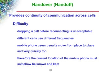
![Erlang B Formula
Determines the probability that a call is blocked
Is a measure of the GOS for trunked systems with blocked
calls cleared
[ ] !
Erlang B formula: GOS
62
A
k
A
C
P blocking C
k
k
C
r = =
å=
0 !](https://image.slidesharecdn.com/thrcellularconcept-141025022958-conversion-gate02/85/Thr-cellular-concept-62-320.jpg)

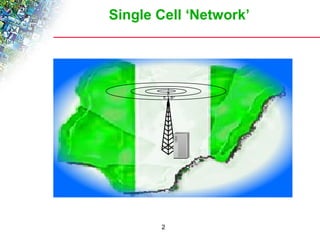
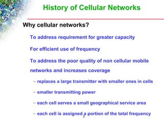
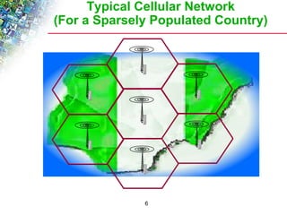
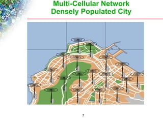
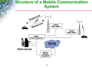
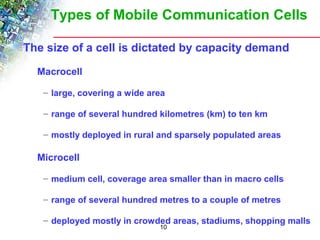
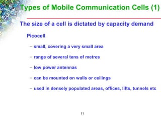
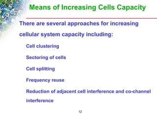
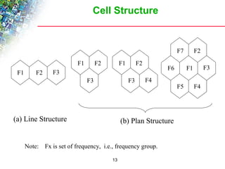
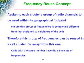
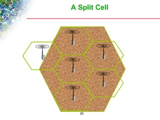
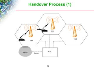
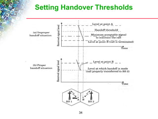
Wireless cellular networks divide geographic areas into smaller sections called cells to improve capacity and coverage. Each cell uses a subset of available frequencies and is served by a base station. As users move between cells, their active connections are handed off between base stations through a process managed by the mobile switching center. Cell sizes and the frequency reuse plan must be optimized to balance capacity, coverage, and interference between cells using the same frequencies.