This document discusses point to point microwave transmission. It describes the basic modules of microwave radio terminals including digital modems, RF units, and passive parabolic antennas. It also covers microwave radio configurations, applications, advantages, planning aspects like network architecture, frequency bands, and propagation effects. Key factors in microwave link engineering like link budgets, reliability predictions, and interference analysis are summarized.

1. Point To Point Microwave Transmission

2. Contents Microwave Radio Basics Radio Network Planning Aspects Radio Network Planning Process Radio wave Propagation Link Engineering & Reliability Interference Analysis PtP MW Transmission Issues Useful Formulae

3. What is Transport ? Transport is an entity that carries information between Network Nodes Information is sent over a carrier between Network Nodes. Carrier is sent over a Transmission Media Commonly used Transmission Media : Copper Cables Microwave Radio Optical Fiber Infra Red Radio

4. Microwave Radio Basics Basic Modules Configuration Applications Advantages

5. Microwave Radio - Modules Microwave Radio Terminal has 3 Basic Modules Digital Modem : To interface with customer equipment and to convert customer traffic to a modulated signal RF Unit : To Up and Down Convert signal in RF Range Passive Parabolic Antenna : For Transmitting and Receiving RF Signal Two Microwave Terminals Forms a Hop Microwave Communication requires LOS

6. Basic Hardware Configurations Non Protected or 1+ 0 Configuration Protected or 1+1 Configuration, also known as MHSB In MHSB Modem and RF Unit are duplicated

7. Microwave Radio – Capacity Configurations Commonly Used Capacity Configurations 4 x 2 Mbps or 4 x E1 8 x 2 Mbps or 8 x E1 16 x 2 Mbps or 16 x E1 155 Mbps or STM1

8. Microwave Radio - Applications As Transport Medium in Basic Service Networks Mobile Cellular Network Last Mile Access Private Networks

9. Microwave Radio Advantages Advantages over Optical Fiber / Copper Cable System Rapid Deployment Flexibility Lower Startup and Operational Cost No ROW Issues Low MTTR

10. Microwave Radio - Manufacturers Few well known Radio Manufacturers Nokia Nera NEC Siemens Digital Microwave Corporation Fujitsu Ericsson Alcatel Hariss

11. Microwave Network Planning Aspects Network Architecture Route Configuration Choice of Frequency Band

12. Network Architecture Common Network Architectures Spur or Chain Star Ring Mesh Combination of Above

13. Spur Architecture B C D E A For N Stations N-1 Links are required Nth station depends on N-1 Links Spur Architecture

14. Star Architecture For N Stations N-1 Links are required Each Station depends on Only 1 Link B C D E A Star Architecture

15. Loop Architecture For N Stations N Links are required Route Diversity is available for all stations B C D E A Loop Architecture

16. Loop protection is effective against faults, which are caused by e.g. power failure equipment failure unexpected cut of cable human mistake rain and multipath fading cutting microwave radio connections

17. BTS DN2 or METROHUB MW RADIO SINGLE MODE MW LINK HSB MODE MW LINK COPPER CONNECTION Figure 2. Primary solution where loop masters (DN2) are co- located in the BSC. To Next BSC To Next BSC BSC

18. Figure 3. Solution of using remote loop master (DN2) co-located in a remote BTS To Next BSC To Next BSC BSC BTS DN2 or METROHUB MW RADIO SINGLE MODE MW LINK HSB MODE MW LINK COPPER CONNECTION

19. Mesh Architecture Each Station is Connected to Every Other Full Proof Route Protection For N sites (Nx2)-1 C D E A Mesh Architecture B

20. Typical Network Architecture B G D E I Typical Architecture J F A C Typical Network Consist of Rings and Spurs

21. Network Routes & Route Capacities Inter- City routes - Backbone Backbone routes are planned at Lower Frequency Bands 2, 6 and 7 GHz Frequency Bands are used Backbone routes are normally high capacity routes Nominal Hop Distances 25 – 40 Km Intra – City routes - Access Access routes are planned at Higher Frequency Bands 15,18 and 23 GHz Frequency Bands are used Nominal Hop Distance 1 – 10 Km

22. Frequency Bands Frequency Band 7, 15, 18 and 23 GHz are allowed to Private Operators for deployment in Transport Network 15,18 and 23 GHz bands are used for Access Network 7 GHz band is used for Backbone Network Different Channeling Plans are available in these bands to accommodate different bandwidth requirements Bandwidth requirement is decided by Radio Capacity offered by the Manufacturer

23. Microwave Propagation

24. Free Space Propagation Microwave Propagation in Free Space is Governed by Laws of Optics Like any Optical Wave , Microwave also undergoes Refraction Reflection

25. Free Space Propagation - Refraction Ray bending due to layers of different densities Bent Rays In Atmosphere

26. Free Space Propagation - Refraction In effect the Earth appears elevated Earth elevation is denoted by K Factor K Factor depends on Rate of Change of Refractivity with height K= 2/3 Earth appears more elevated K= 4/3 Earth appears flatter w.r.t K=2/3 K=  Ray Follows Earth Curvature

27. Free Space Propagation - Refraction Effect of Refractivity Change K = 2/3 Actual Ground K = 4/3

28. Microwaves are reflected over Smooth Surfaces Water Bodies Reflected Signals are 180  out of phase Reflection can be a major cause of outages Link needs to be planned carefully to avoid reflections Free Space Propagation – Reflections

29. RF Propagation Reflections Reflections can come from ANYWHERE - behind, under, in-front 6 cm difference can change Path geometry

30. Fresnel Zone The Fresnel zone is the area of space between the two antennas in which the radio signal travels. For Clear Line of Sight Fresnel Zone Should be clear of obstacles It is depands on Distance and Frequency

31. FRESNEL ZONES 1st Fresnel Zone Mid Path

32. FRESNEL ZONE CLEARANCES 1 ST Fresnal Zone = 17.3  (d1*d2)/f(d1+d2) d1 = Distance in Kilometers from Antenna ‘A’ to mid point d2 = Distance in Kilometers from Antenna ‘B’ to mid point f = Frequency in GHz A d1 d2 B

33. RF propagation First Fresnel Zone

34. RF propagation Free space versus non free space Non-free space Line of sight required Objects protrude in the fresnel zone, but do not block the path Free Space Line of sight No objects in the fresnel zone Antenna height is significant Distance relative short (due to effects of curvature of the earth)

35. FRESNEL ZONE & EARTH BULGE D 2 /8 Earth Bulge Height = D 2 /8 + 43.3  D/4F 43.3  D/4F 60% first Fresnel Zone D = Distance Between Antennas H

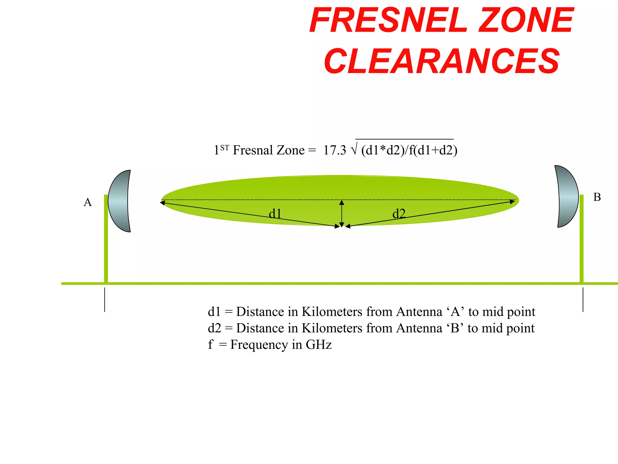
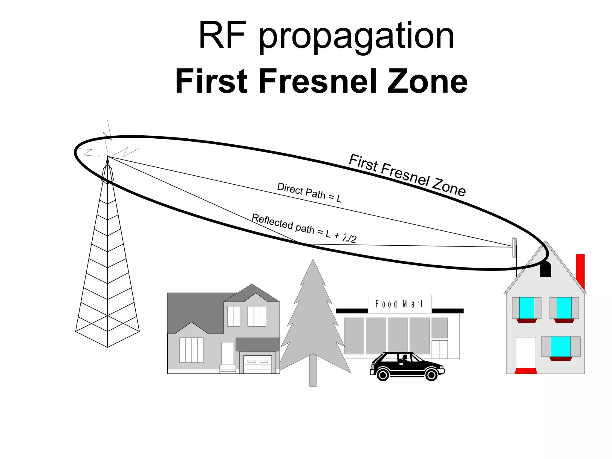
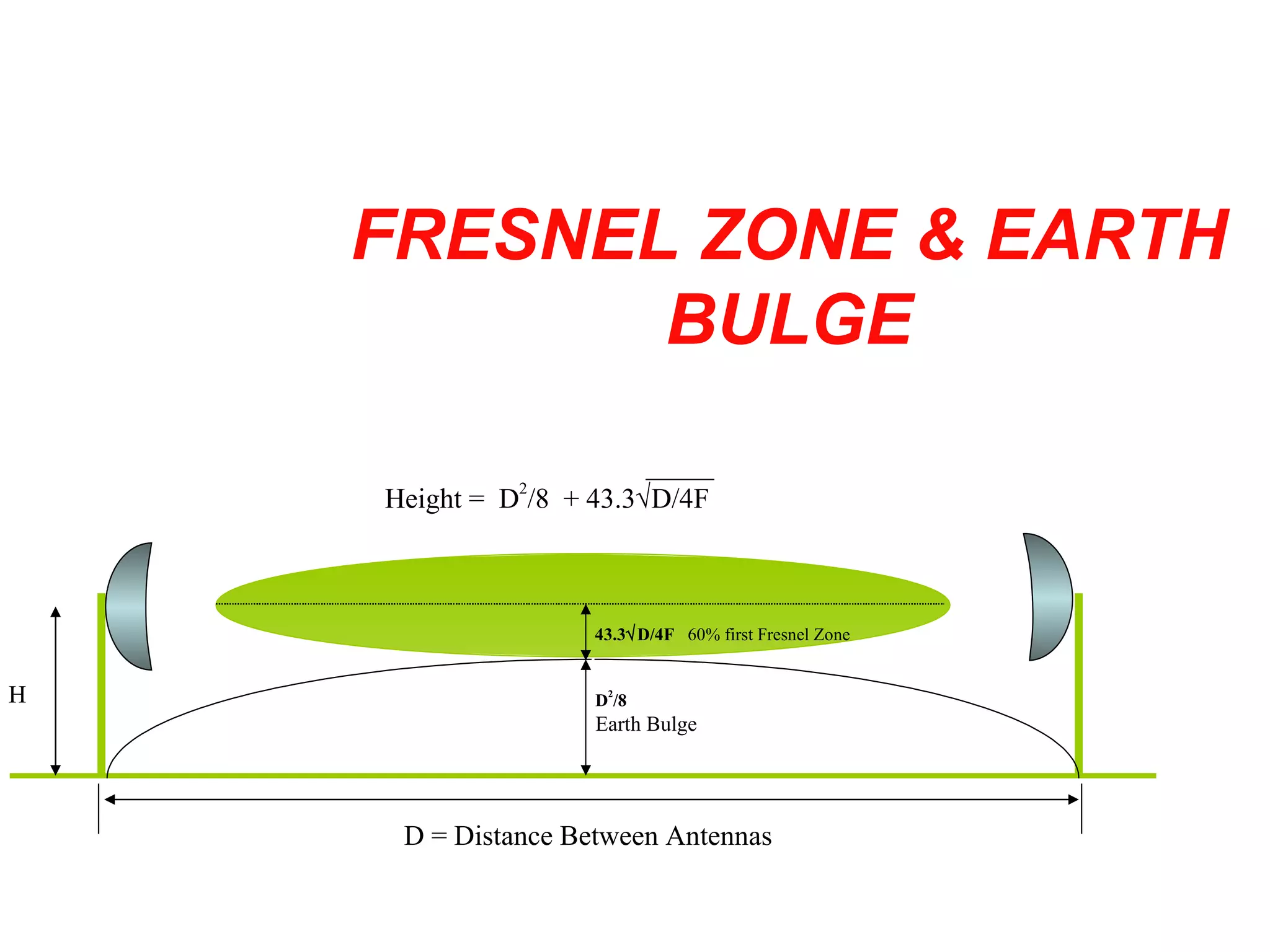
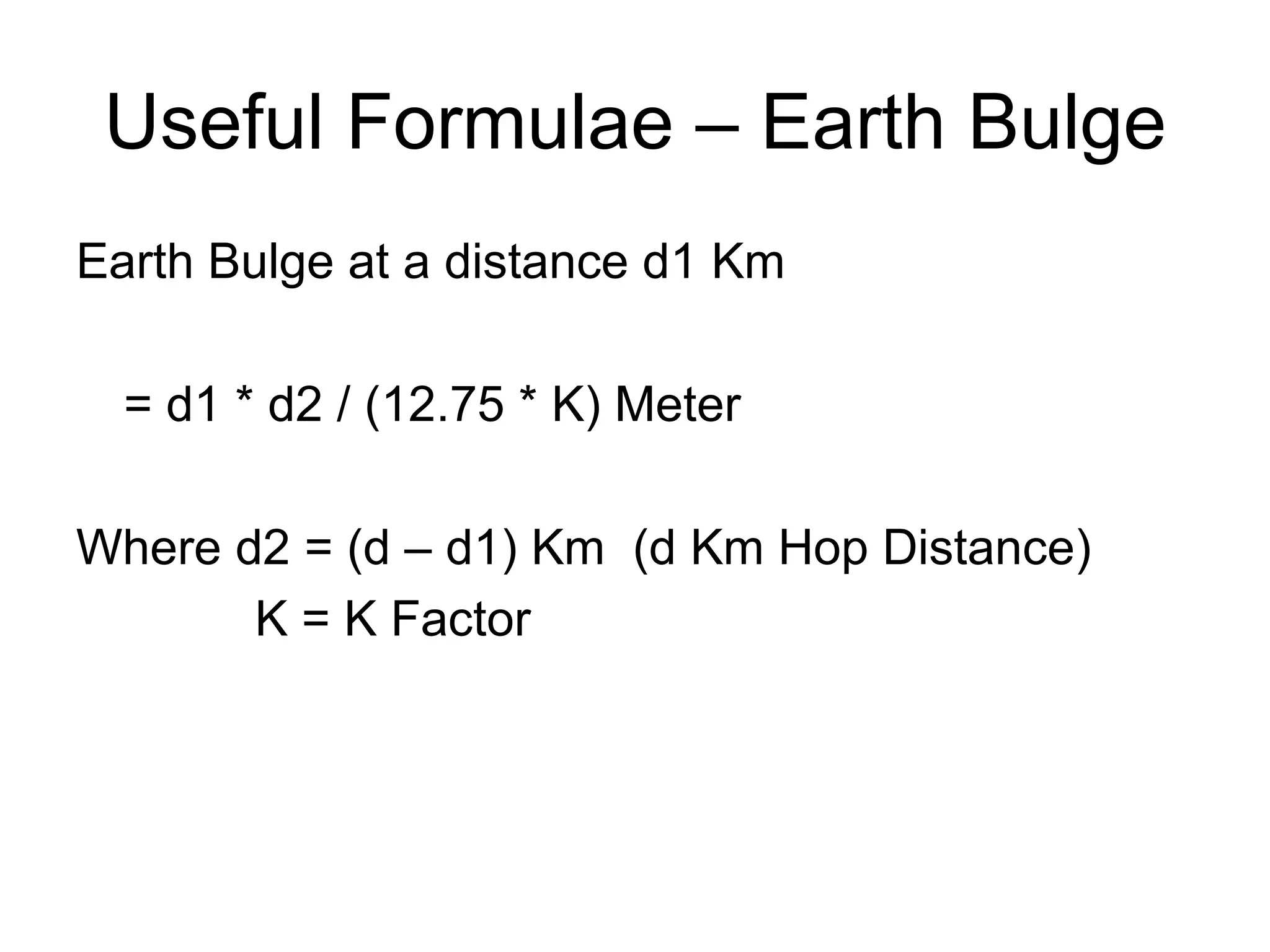
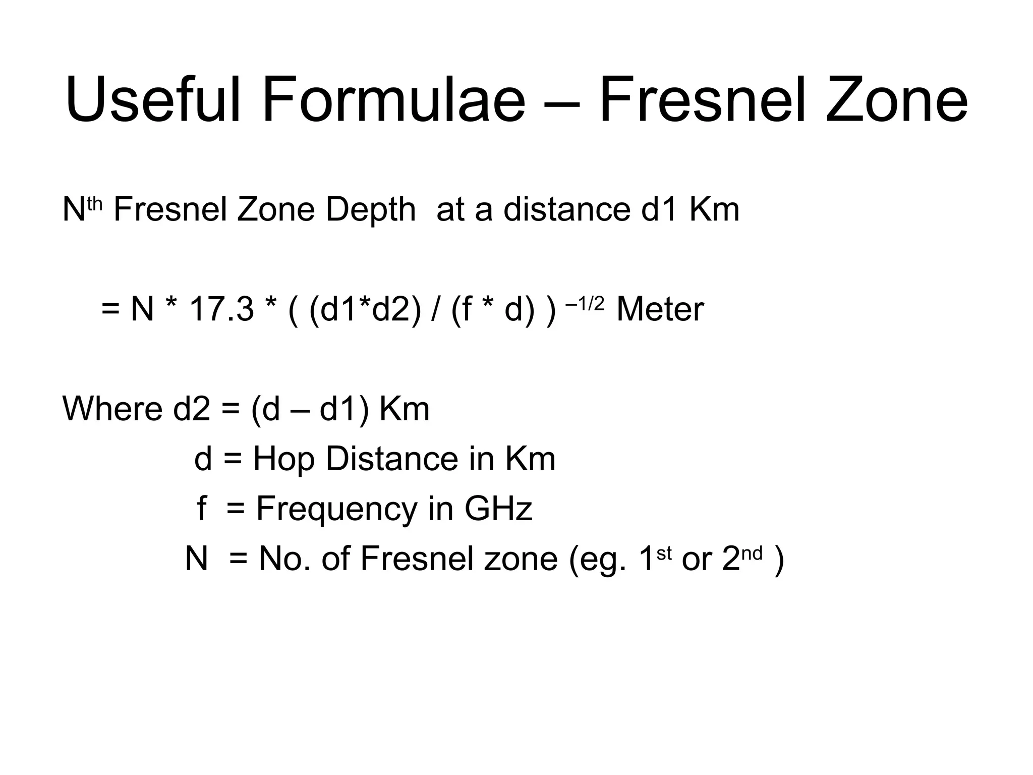
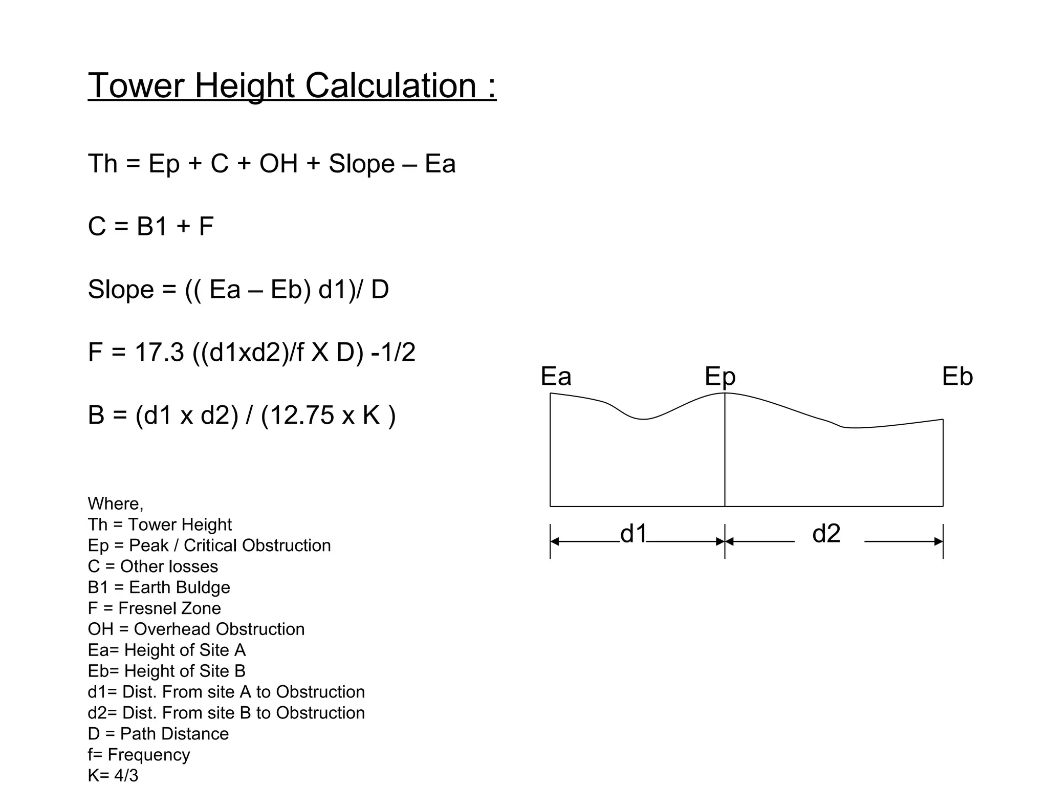
36. Midpoint clearance = 0.6F + Earth curvature + 10' when K=1 First Fresnel Distance (meters) F1= 17.3 [(d1*d2)/(f*D)] 1/2 where D=path length Km, f=frequency (GHz) , d1= distance from Antenna1(Km) , d2 = distance from Antenna 2 (Km) Earth Curvature h = (d1*d2) /2 where h = change in vertical distance from Horizontal line (meters), d1&d2 distance from antennas 1&2 respectively Clearance for Earth’s Curvature 13 feet for 10 Km path 200 feet for 40 Km path Fresnel Zone Clearance = 0.6 first Fresnel distance (Clear Path for Signal at mid point) 30 feet for 10 Km path 57 feet for 40 Km path RF Propagation Antenna Height requirements Earth Curvature Obstacle Clearance Fresnel Zone Clearance Antenna Height Antenna Height

37. Microwave Network Planning Process Design Basis Line of Sight Survey Link Engineering Interference Analysis

38. N N Y Y RF Nominal Planning (NP)/ Application for Frequency License Define BSC Borders Estimate BSC Locations Preliminary Transmission Planning and LOS Checking for possible BSCs Finalize BSC Locations Microwave Link Planning and LOS Checking for BTSs Update LOS Reports, Frequency Plan, Planning Database, Equipment Summary Customer to apply SACFA based on Nokia Technical Inputs Change BTS Prime Candidate? Change BTS Prime Candidate? Figure 1. Microwave Link Planning Process Planning Process

39. Design Basis Choice of Radio Equipment Fresnel Zone Clearance Objectives Availability / Reliability Objectives Interference Degradation Objectives Tower Height & Loading Restrictions

40. Microwave Network Planning Process Map Study for feasibility of Line of Sight and Estimating Tower Heights Actual Field Survey for refining map data and finalizing Antenna Heights Link Power Budgeting & Engineering Frequency and Polarization Assignments Interference Analysis (Network Level) Final Link Engineering (Network Level)

41. Map Study SOI Maps are available in different Scales and Contour Intervals 1:50000 Scale Maps with 20 M Contour Interval are normally used for Map Study Sites are Plotted on Map Contour values are noted at intersections Intersection with Water Bodies is also noted AMSL of Sight is determined by Interpolation

42. Map Study Vegetation height (15-20m) is added to Map Data Path Profile is drawn on Graph for Earth Bulge Factor (K) =4/3 and 2/3 Fresnel Zone Depths are Calculated & Plotted for Design Frequency Band Antennae Heights are Estimated for Design Clearance Criteria

43. Field Survey Equipment Required Data Required GPS Receiver - Map Study Data Camera Magnetic Compass Altimeter Binocular / Telescope Flashing Mirror Flags Inclinometer Balloon Set Measuring Tapes

44. Field Survey Field Survey Map Data Validation Gathering Field inputs (Terrain Type, Average Tree/Obstacle Height, Critical Obstruction etc.) Line of Sight Check, if feasible ,using flags, mirror Data related to other stations in the vicinity , their coordinates, frequency of operation, antenna size, heights, power etc. Proximity to Airport / Airstrip with their co-ordinates Field inputs are used to refine existing path profile data , reflection point determination, reflection analysis

45. RF propagation Environmental conditions Line of Sight No objects in path between antenna a. Neighboring Buildings b. Trees or other obstructions Interference c. Power lines

46. Fading Phenomenon of Attenuation of Signal Due to Atmospheric and Propagation Conditions is called Fading Fading can occur due to Refractions Reflections Atmospheric Anomalies

47. Fading Types of Fading Multipath Fading Frequency Selective Fading Rain Fading

48. Multipath Fading Multipath fading is caused due to reflected / refracted signals arriving at receiver Reflected Signals arrive with Delay Phase Shift Result in degradation of intended Signal Space Diversity Radio Configuration is used to Counter Multipath Fading

49. Frequency Selective Fading Frequency Selective Fading Due to Atmospheric anomalies different frequencies undergo different attenuation levels Frequency Diversity Radio Configuration is used to Counter Frequency Selective Fading

50. Rain Fading Frequency Band > 10 GHz are affected due to Rain as Droplet size is comparable to Wavelengths Rain Fading Occur over and above Multipath and Frequency Selective Fading Horizontal Polarization is more prone to Rain Fades Path Diversity / Route Diversity is the only counter measure for Rain Fade

51. Drop Shape and Polarization 2.0mm 1mm 1.5mm 2.5mm As raindrops increase in size, they get more extended in the Horizontal direction, and therefore will attenuate horizontal polarization more than vertical polarization

52. Fade Margin Margin required to account for Fading – Fade Margin Higher Fade Margin provide better Link Reliability Fade Margin of 35 – 40 dB is normally provided

53. Link Engineering & Reliability Link Budgeting Reliability Predictions Interference Analysis

54. Hop Model Outdoor Unit Station B Indoor Unit Traffic Outdoor Unit Station A Indoor Unit Traffic

55. Link Power Budget Received Signal Level = R xl R xlB = T xA – L A + G A – F l + G B – L B Where T XA = Trans Power Station A L A = Losses at Station A (Misc.) G A = Antenna Gain at Station A F l = Free Space Losses G B = Antenna Gain at Station B L B = Losses at Station B R xlB = Rx. Level at Station B R XL must be > Receiver Sensitivity always

56. Link Power Budget – Receiver Sensitivity Lowest Possible Signal which can be detected by Receiver is called Receiver Sensitivity or Threshold Threshold Value is Manufacturer Specific Depends on Radio Design Higher (-ve) Value Indicates better Radio Design

57. Link Engineering Software Tools are used Inputs to the tool Sight Co-ordinates Path Profile Data Terrain Data & Rain Data Equipment Data Antenna Data Frequency and Polarization Data Tool Output Availability Prediction

58. RF propagation Simple Path Analysis Concept (alternative) WP II PC Card pigtail cable Lightning Protector RF Cable Antenna WP II PC Card pigtail cable Lightning Protector RF Cable Antenna + Transmit Power - LOSS Cable/connectors + Antenna Gain + Antenna Gain - LOSS Cable/connectors RSL ( receive signal level) + Fade Margin = sensitivity - Path Loss over link distance Calculate signal in one direction if Antennas and active components are equal

59. Link Engineering – Interference Interference is caused due to undesirable RF Signal Coupling Threshold is degraded due to interference Degraded Threshold results in reduced reliability

60. Link Engineering – Interference Examples of Undesirable RF Couplings Finite Value of XPD in Antenna is the Prime Cause Solution : Use of High Performance Antenna F 1 H V Cross Poler Coupling

61. Link Engineering – Interference Examples of Undesirable RF Coupling Receiver Filter Cut-off is tappered Solution : Use Radio with better Specifications F 2 Adjacent Channel F 1

62. Link Engineering – Interference Examples of Undesirable RF Coupling Finite value of FTB Ratio of Antenna is Prime Cause Solution : Antenna with High FTB Ratio Front to Back T : Hi R : Low T : Hi R : Low T : Low R : Hi T : Low R : Hi

63. Link Engineering – Interference Examples of Undesirable RF Coupling Solution : Choose Antenna Heights such a way there is no LOS for over reach Over Reach T : Low R : Hi T : Hi R : Low T : Hi R : Low T : Low R : Hi T : Low R : Hi T : Hi R : Low

64. Link Engineering – Interference Interference is calculated at Network Level Interference due to links Within Network Outside Network (Links of other Operators) Interfering Signal degrades Fade Margin Engineering Calculation re-done with degraded Fade Margin

65. Link Engineering – Interference Counter Measures Avoid Hi-Lo violation in loop Frequency Discrimination Polarization Discrimination Angular Discrimination High Performance Antennae Lower Transmit Power , if possible

66. DN2 PORT ALLOCATION: ET (Exchange Terminal) Port DN2 Port DN2 to Network connection DN2 to BSC Connection P20 P18 P16 P14 P12 P10 P8 P6 P4 P2 P19 P17 P15 P13 P11 P9 P7 P5 P3 P1 DN2 20 Port

67. BTS4 ET33 STANDARD MICROWAVE RADIO FIU 19 TRIBUTARY ALLOCATION FOR LOOP PROTECTION BSC DN2 2 BTS7 BTS6 BTS5 BTS3 BTS2 BTS1 BTS8 ET32 ET33 ET34 ET32 ET34 ET35 ET35

68. FIU 1 FIU2 FB1 FB2 FB1 FB2 LOOP 1 LOOP2 Loop Protection with Hardware Protection

69. PtP Microwave Transmission - Issues Link Performance is Seriously Affected due to Atmospheric Anomalies like Ducting Ground Reflections Selective Fading Excessive Rains Interferences Thunderstorms / High Winds causing Antenna Misalignment Earthing Equipment Failure

70. Some Useful Formulae

71. Link Budget Rx B A B +GA +GB -Lfs-Arain B Rain fs A A B G A L G Tx Rx      +Tx A

72. d=1km ---> L = 124 dBm d=2km ---> L = 130 dBm d=1km ---> L = 121 dBm d=2km ---> L = 127 dBm 39 GHz 26 GHz Examples Free Space Loss d = distance in kilometers f = frequency in GHz

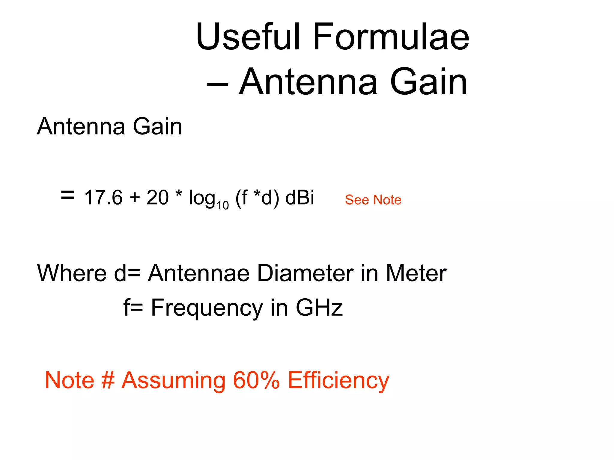
73. RF Propagation Basic loss formula Propagation Loss d = distance between Tx and Rx antenna [meter] P T = transmit power [mW] P R = receive power [mW] G = antennae gain Pr ~ 1/f 2 * D 2 which means 2X Frequency = 1/4 Power 2 X Distance = 1/4 Power

74. Useful Formulae – Earth Bulge Earth Bulge at a distance d1 Km = d1 * d2 / (12.75 * K) Meter Where d2 = (d – d1) Km (d Km Hop Distance) K = K Factor

75. Useful Formulae – Fresnel Zone N th Fresnel Zone Depth at a distance d1 Km = N * 17.3 * ( (d1*d2) / (f * d) ) –1/2 Meter Where d2 = (d – d1) Km d = Hop Distance in Km f = Frequency in GHz N = No. of Fresnel zone (eg. 1 st or 2 nd )

76. Tower Height Calculation : Th = Ep + C + OH + Slope – Ea C = B1 + F Slope = (( Ea – Eb) d1)/ D F = 17.3 ((d1xd2)/f X D) -1/2 B = (d1 x d2) / (12.75 x K ) Where, Th = Tower Height Ep = Peak / Critical Obstruction C = Other losses B1 = Earth Buldge F = Fresnel Zone OH = Overhead Obstruction Ea= Height of Site A Eb= Height of Site B d1= Dist. From site A to Obstruction d2= Dist. From site B to Obstruction D = Path Distance f= Frequency K= 4/3 d1 d2 Ea Ep Eb

77. Useful Formulae – Antenna Gain Antenna Gain = 17.6 + 20 * log 10 (f *d) dBi See Note Where d= Antennae Diameter in Meter f= Frequency in GHz Note # Assuming 60% Efficiency

78. Useful Formulae – Free Space Loss Free Space Loss F l = 92.4 + 20 * log 10 (f *d) dB Where d = Hop Distance in Km f = Frequency in GHz

79. Useful Formulae – Geo Climatic Factor Geo Climatic Factor G = 10 –T * (P l ) 1.5 Where T= Terrain Factor = 6.5 for Overland Path Not in Mountain = 7.1 for Overland Path in Mountain = 6.0 for Over Large Bodies of Water P l = P l factor

80. Useful Formulae – System Gain System Gain = (Transmit Power + ABS(Threshold) ) dB Fade Margin = FM = (Nominal Received Signal – Threshold) dB Path Inclination  = ABS ((h 1 + A 1 ) – (h 2 + A 2 ) ) / d Where h1 = Ant. Ht. At Stn A AGL Meter h2 = Ant. Ht. At Stn B AGL Meter A1 = AMSL of Stn A Meter A2 = AMSL of Stn B Meter d = Hop Distance in KM

81. Useful Formulae – Fade Occurrence Factor Fade Occurrence Factor =   = G * d 3.6 *f 0.89 * (1+  ) -1.4 Where G = Geo Climatic Factor d = Hop Distance in Km f = Frequency in GHz  = Path Inclination in mRad

82. Useful Formulae – Outage Probability Worst Month Outage Probability (One Way) % = O WM O WM % =  * 10 –(FM/10) Annual Unavailability (One Way) % = O WM * 0.3 Assuming 4 Worst Months in a Year Annual Availability (Two Way) % = 100-(O WM *0.3*2)