heap sort ppt for university studetn

1. Introduction to Algorithms
Chapter 6: Heap Sort

2. 5
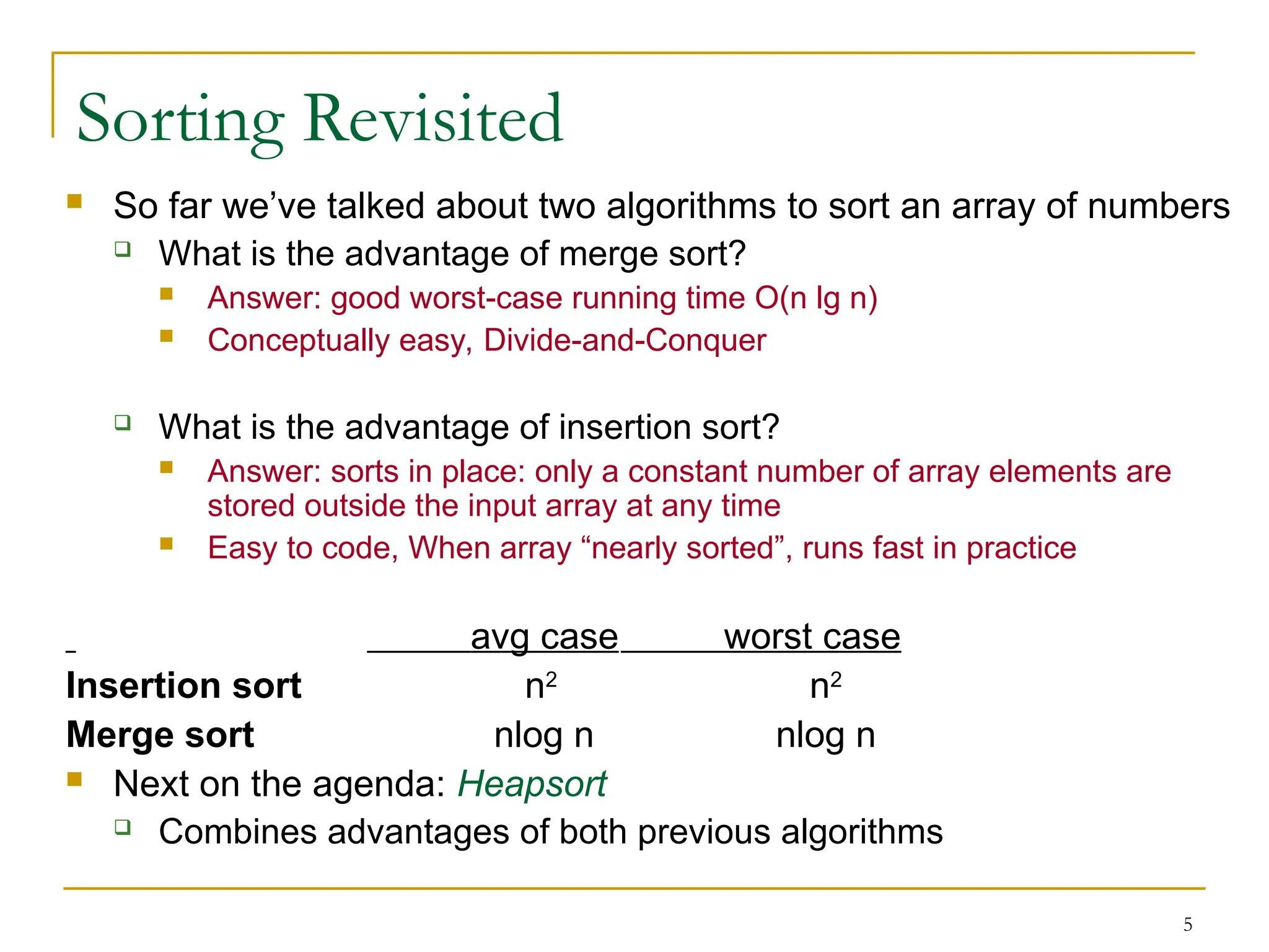
Sorting Revisited
 So far we’ve talked about two algorithms to sort an array of numbers
 What is the advantage of merge sort?
 Answer: good worst-case running time O(n lg n)
 Conceptually easy, Divide-and-Conquer
 What is the advantage of insertion sort?
 Answer: sorts in place: only a constant number of array elements are
stored outside the input array at any time
 Easy to code, When array “nearly sorted”, runs fast in practice
avg case worst case
Insertion sort n2
n2
Merge sort nlog n nlog n
 Next on the agenda: Heapsort
 Combines advantages of both previous algorithms

3. 6
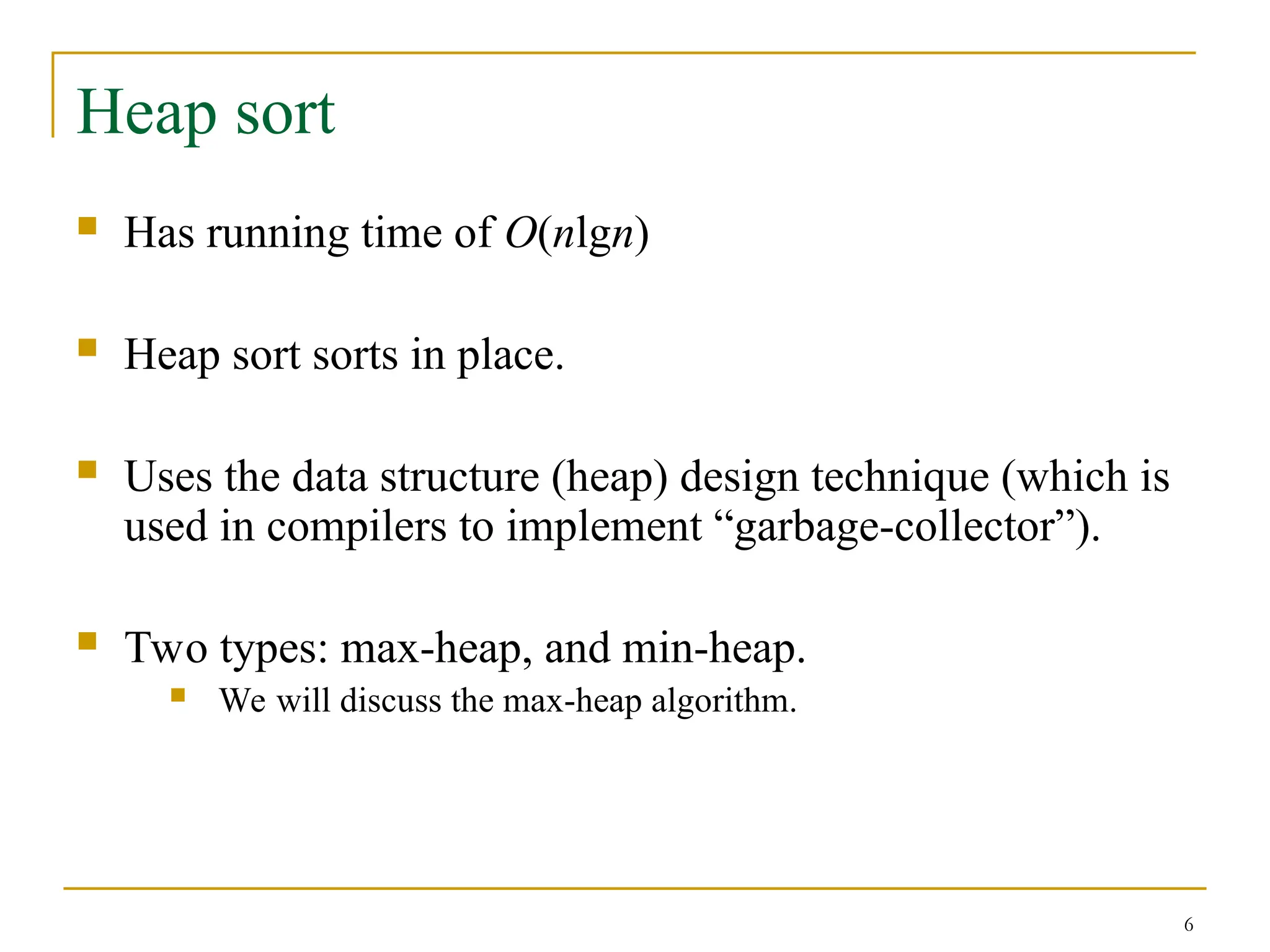
Heap sort
 Has running time of O(nlgn)
 Heap sort sorts in place.
 Uses the data structure (heap) design technique (which is
used in compilers to implement “garbage-collector”).
 Two types: max-heap, and min-heap.
 We will discuss the max-heap algorithm.

4. 7
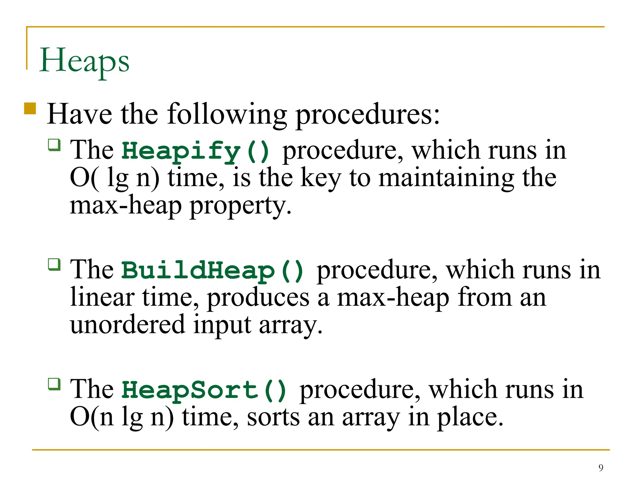
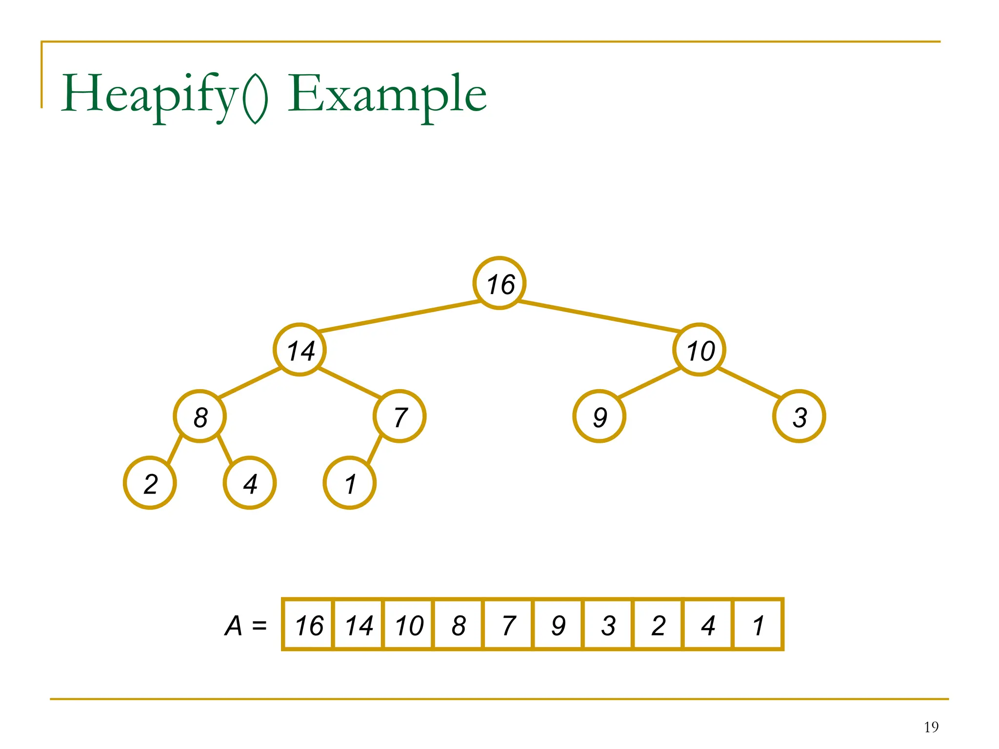
Heaps
 A heap can be seen as a complete binary tree
 The tree is completely filled on all levels except possibly the lowest.
 In practice, heaps are usually implemented as arrays
 An array A that represent a heap is an object with two attributes:
A[1 .. length[A]]
 length[A]: # of elements in the array
 heap-size[A]: # of elements in the heap stored within array A, where
heap-size[A] ≤ length[A]
 No element past A[heap-size[A]] is an element of the heap
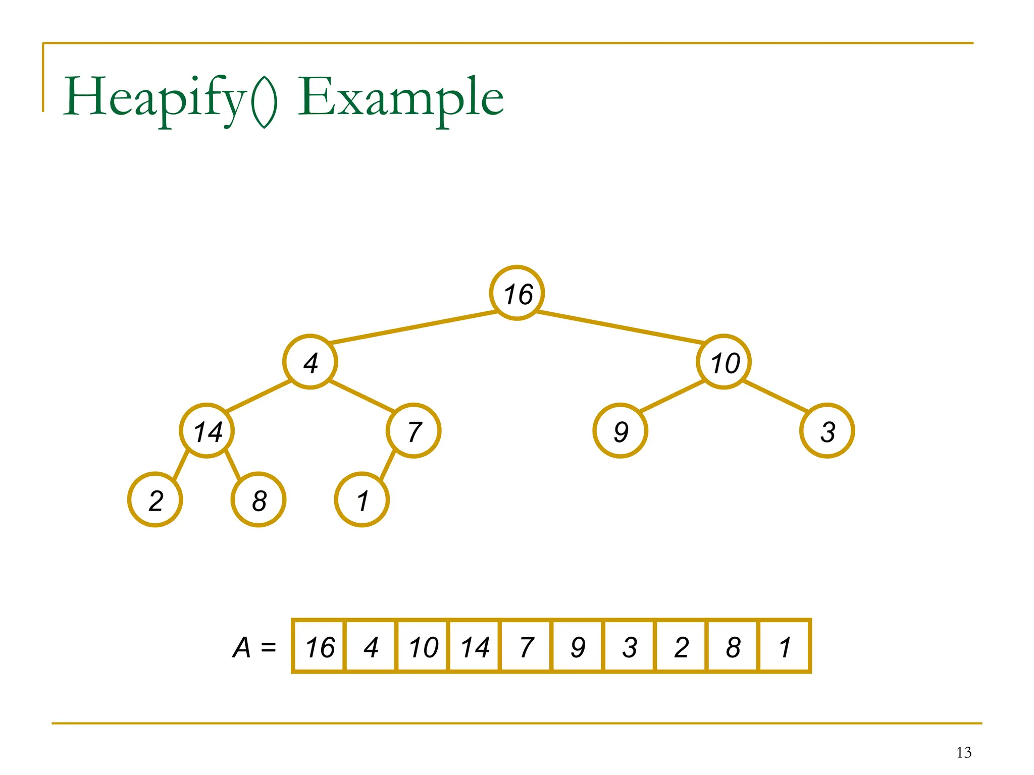
16 14 10 8 7 9 3 2 4 1
A =

5. 8
Referencing Heap Elements
 The root node is A[1]
 Node i is A[i]
 Parent(i)
 return i/2
 Left(i)
 return 2*i
 Right(i)
 return 2*i + 1
1
2
3
4
5
6
7
8
9
10
16
15
10
8
7
9
3
2
4
1
Level: 3 2 1 0

6. 9
Heaps
 Have the following procedures:
 The Heapify() procedure, which runs in
O( lg n) time, is the key to maintaining the
max-heap property.
 The BuildHeap() procedure, which runs in
linear time, produces a max-heap from an
unordered input array.
 The HeapSort() procedure, which runs in
O(n lg n) time, sorts an array in place.

7. 10
The Heap Property
 Heaps also satisfy the heap property (max-
heap):
 A[Parent(i)]  A[i] for all nodes i > 1
 In other words, the value of a node is at most the
value of its parent
 The largest value in a heap is at its root (A[1])
 and subtrees rooted at a specific node contain
values no larger than that node’s value

8. 11
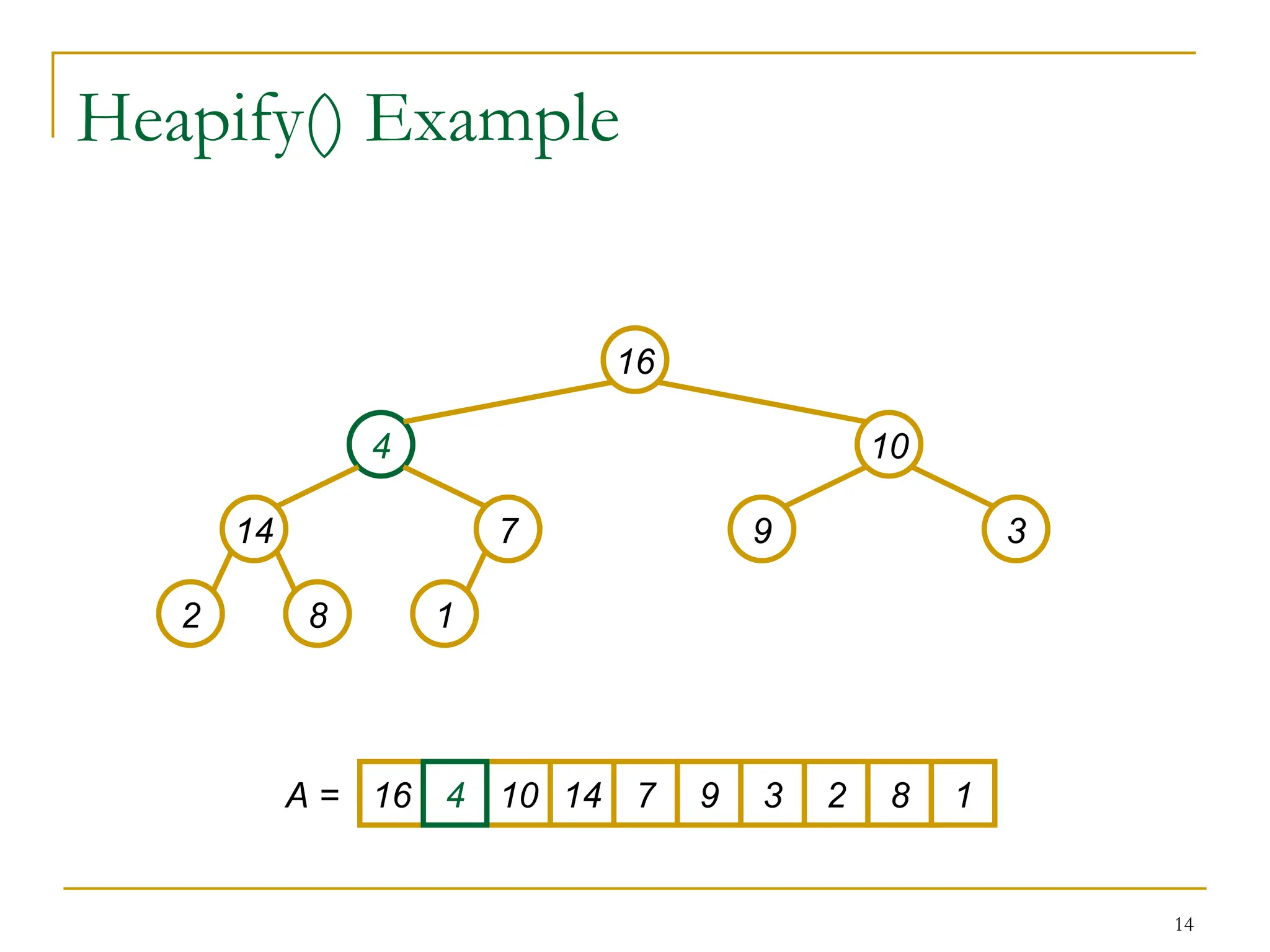
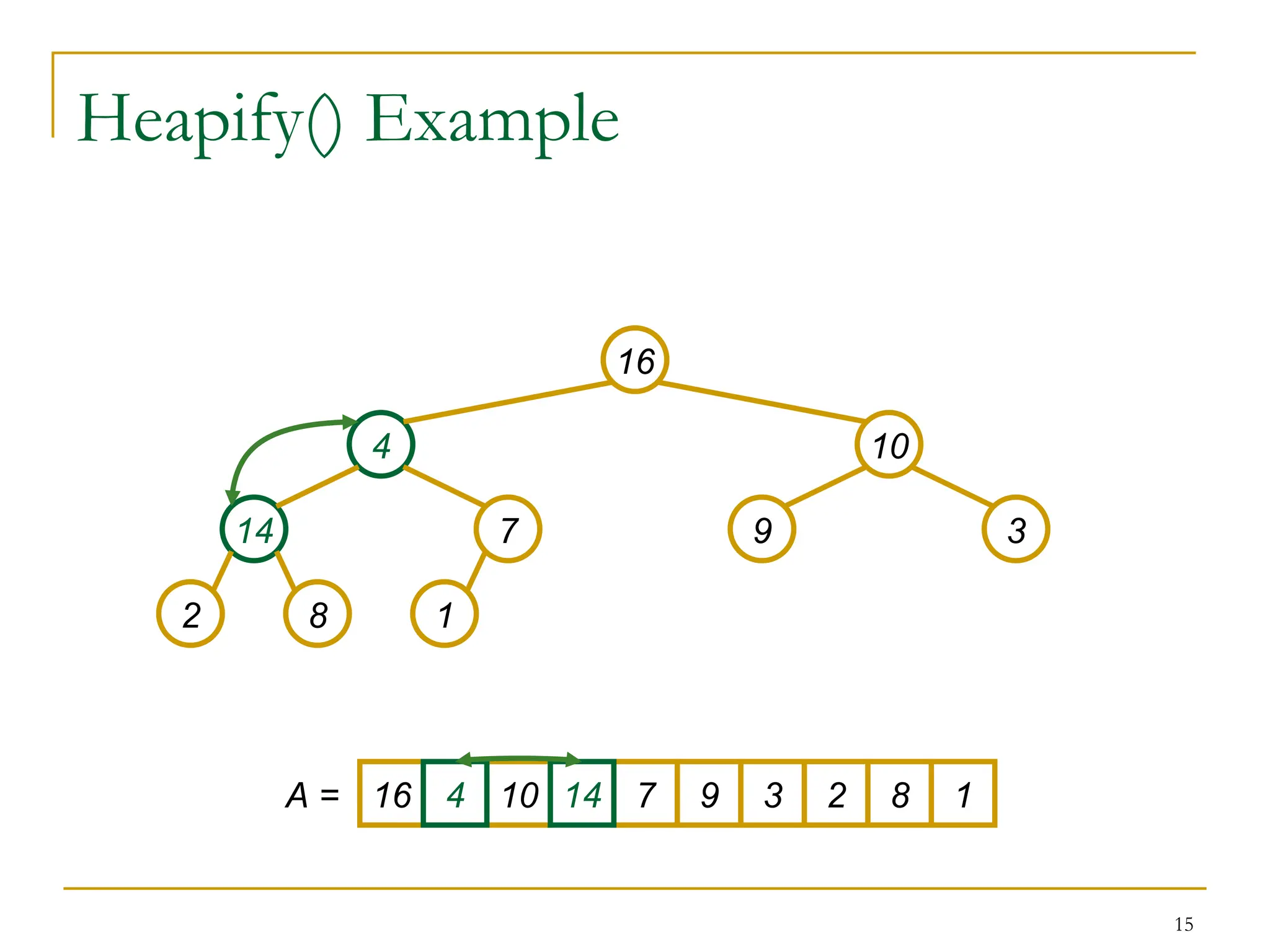
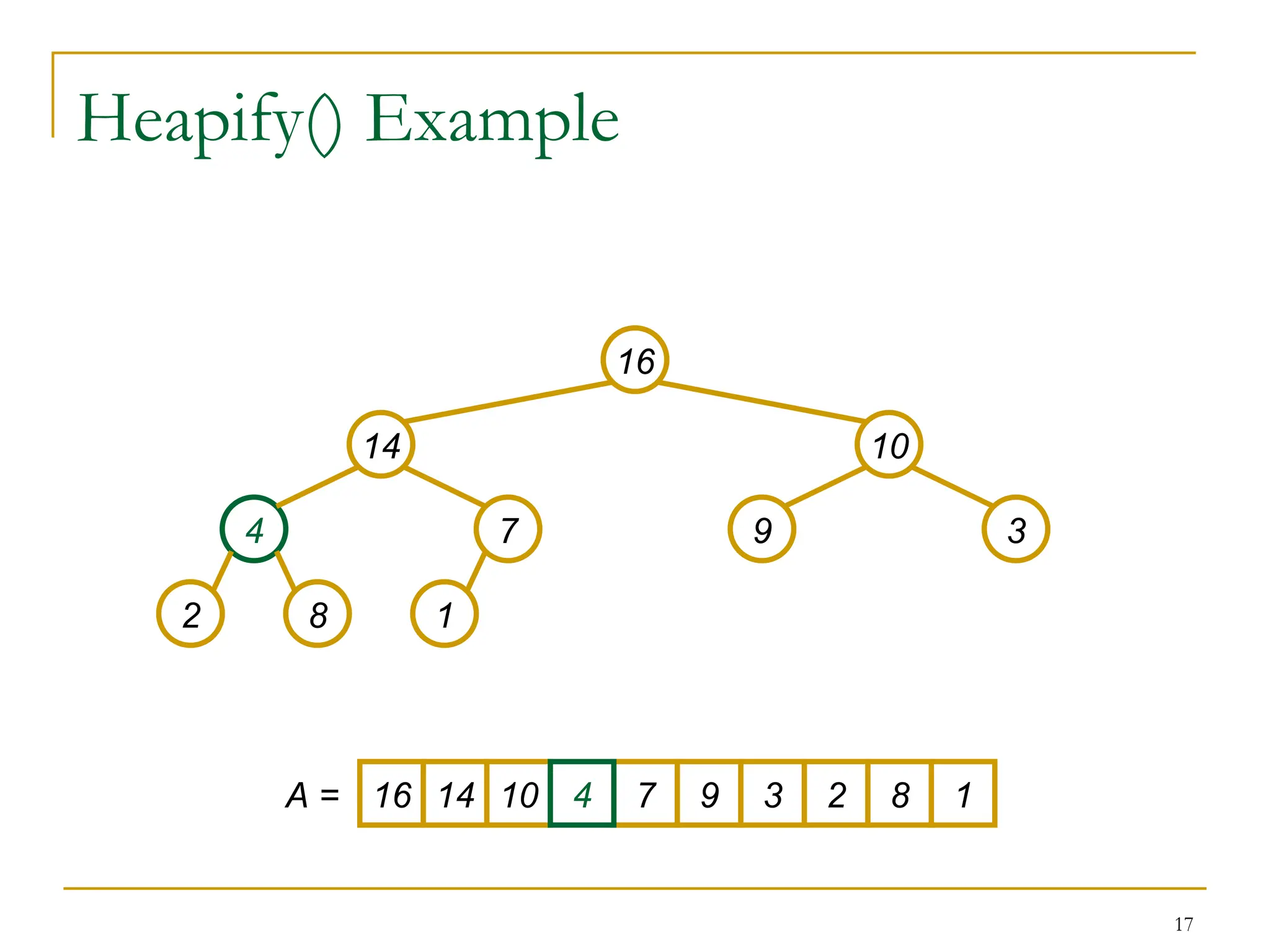
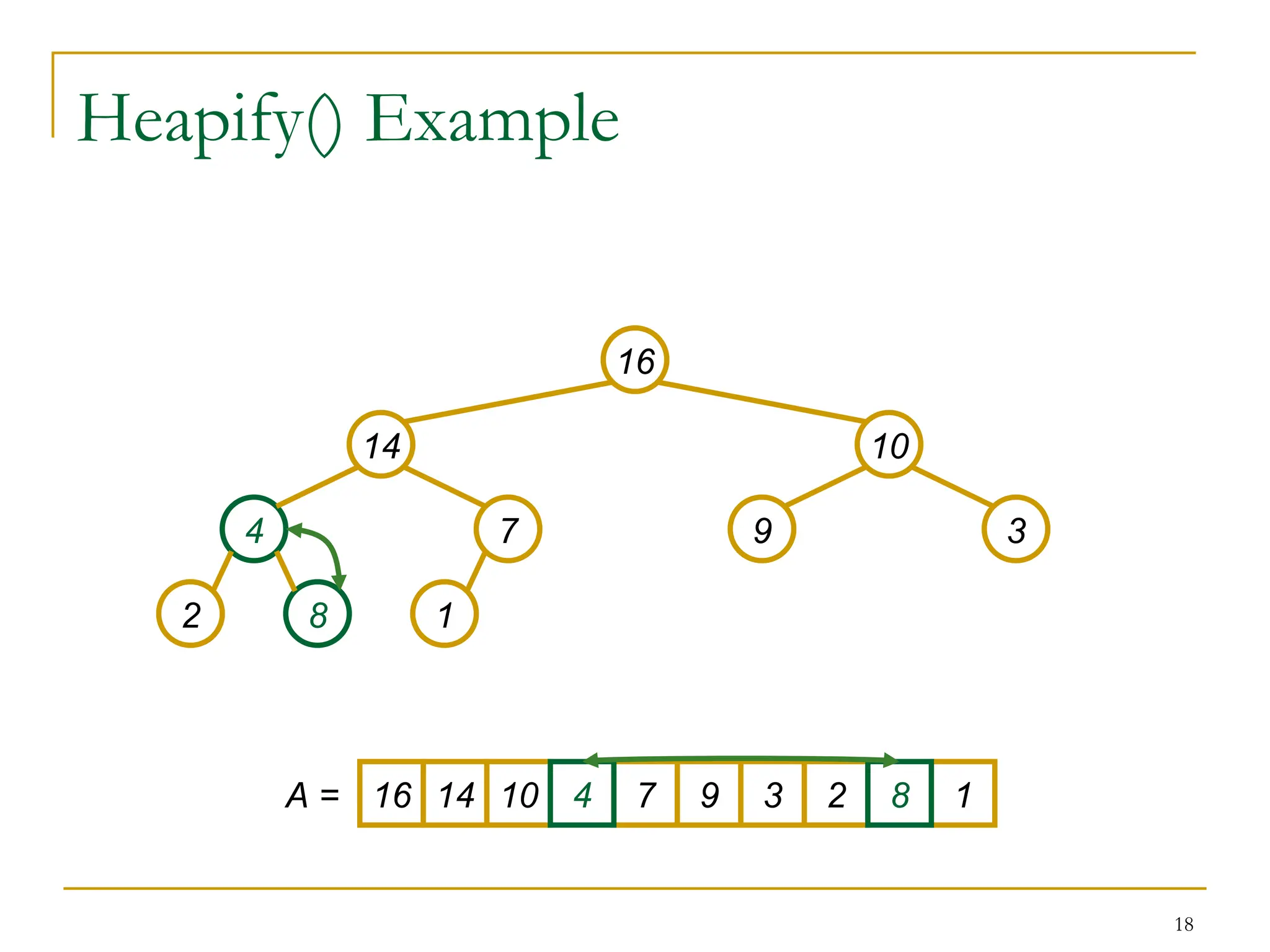
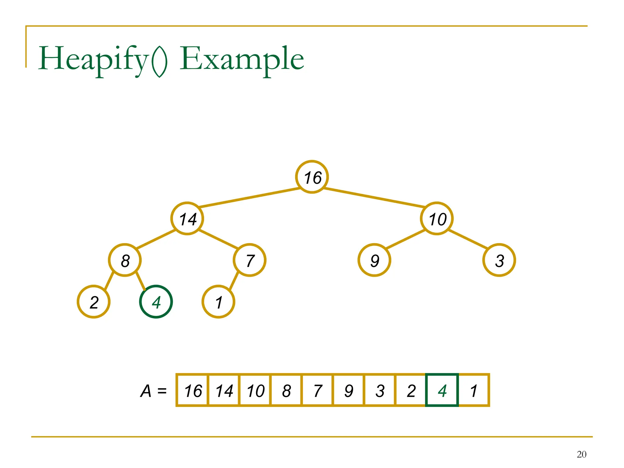
Heap Operations: Heapify
)(
 Heapify(): maintain the heap property
 Given: a node i in the heap with children L and R
 two subtrees rooted at L and R, assumed to be
heaps
 Problem: The subtree rooted at i may violate the heap
property (How?)
 A[i] may be smaller than its children value
 Action: let the value of the parent node “float down” so
subtree at i satisfies the heap property
 If A[i] < A[L] or A[i] < A[R], swap A[i] with the
largest of A[L] and A[R]
 Recurs on that subtree

9. 12
Heap Operations: Heapify
)(
Heapify(A, i)
{
1. L  left(i)
2. R  right(i)
3. if L  heap-size[A] and A[L] > A[i]
4. then largest  L
5. else largest  i
6. if R  heap-size[A] and A[R] > A[largest]
7. then largest  R
8. if largest i
9. then exchange A[i]  A[largest]
10. Heapify(A, largest)
}

10. 13
Heapify() Example
16
4 10
14 7 9 3
2 8 1
16 4 10 14 7 9 3 2 8 1
A =

11. 14
Heapify() Example
16
4 10
14 7 9 3
2 8 1
16 10 14 7 9 3 2 8 1
A = 4

12. 15
Heapify() Example
16
4 10
14 7 9 3
2 8 1
16 10 7 9 3 2 8 1
A = 4 14

13. 16
Heapify() Example
16
14 10
4 7 9 3
2 8 1
16 14 10 4 7 9 3 2 8 1
A =

14. 17
Heapify() Example
16
14 10
4 7 9 3
2 8 1
16 14 10 7 9 3 2 8 1
A = 4

15. 18
Heapify() Example
16
14 10
4 7 9 3
2 8 1
16 14 10 7 9 3 2 1
A = 4 8

16. 19
Heapify() Example
16
14 10
8 7 9 3
2 4 1
16 14 10 8 7 9 3 2 4 1
A =

17. 20
Heapify() Example
16
14 10
8 7 9 3
2 4 1
16 14 10 8 7 9 3 2 1
A = 4

18. 21
Heapify() Example
16
14 10
8 7 9 3
2 4 1
16 14 10 8 7 9 3 2 4 1
A =

19. 22
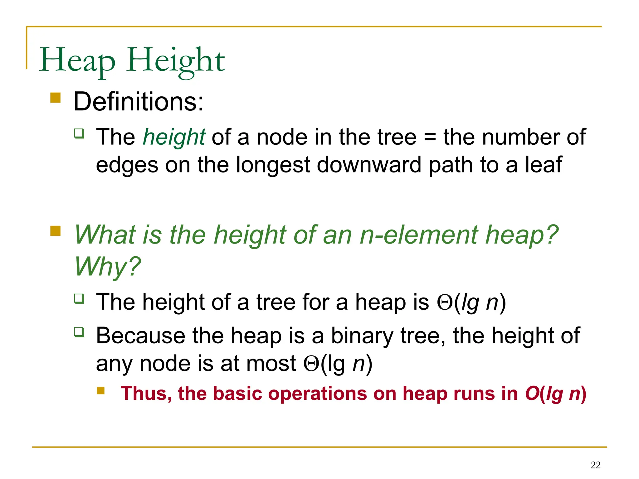
Heap Height
 Definitions:
 The height of a node in the tree = the number of
edges on the longest downward path to a leaf
 What is the height of an n-element heap?
Why?
 The height of a tree for a heap is (lg n)
 Because the heap is a binary tree, the height of
any node is at most (lg n)
 Thus, the basic operations on heap runs in O(lg n)

20. 23
#
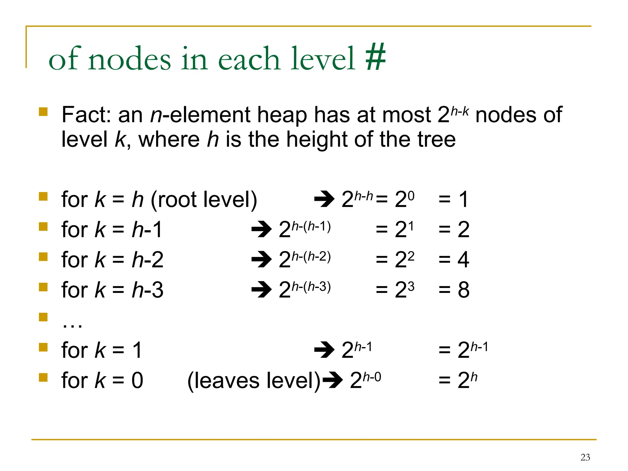
of nodes in each level
 Fact: an n-element heap has at most 2h-k
nodes of
level k, where h is the height of the tree
 for k = h (root level)  2h-h
= 20
= 1
 for k = h-1  2h-(h-1)
= 21
= 2
 for k = h-2  2h-(h-2)
= 22
= 4
 for k = h-3  2h-(h-3)
= 23
= 8
 …
 for k = 1  2h-1
= 2h-1
 for k = 0 (leaves level) 2h-0
= 2h

21. 24
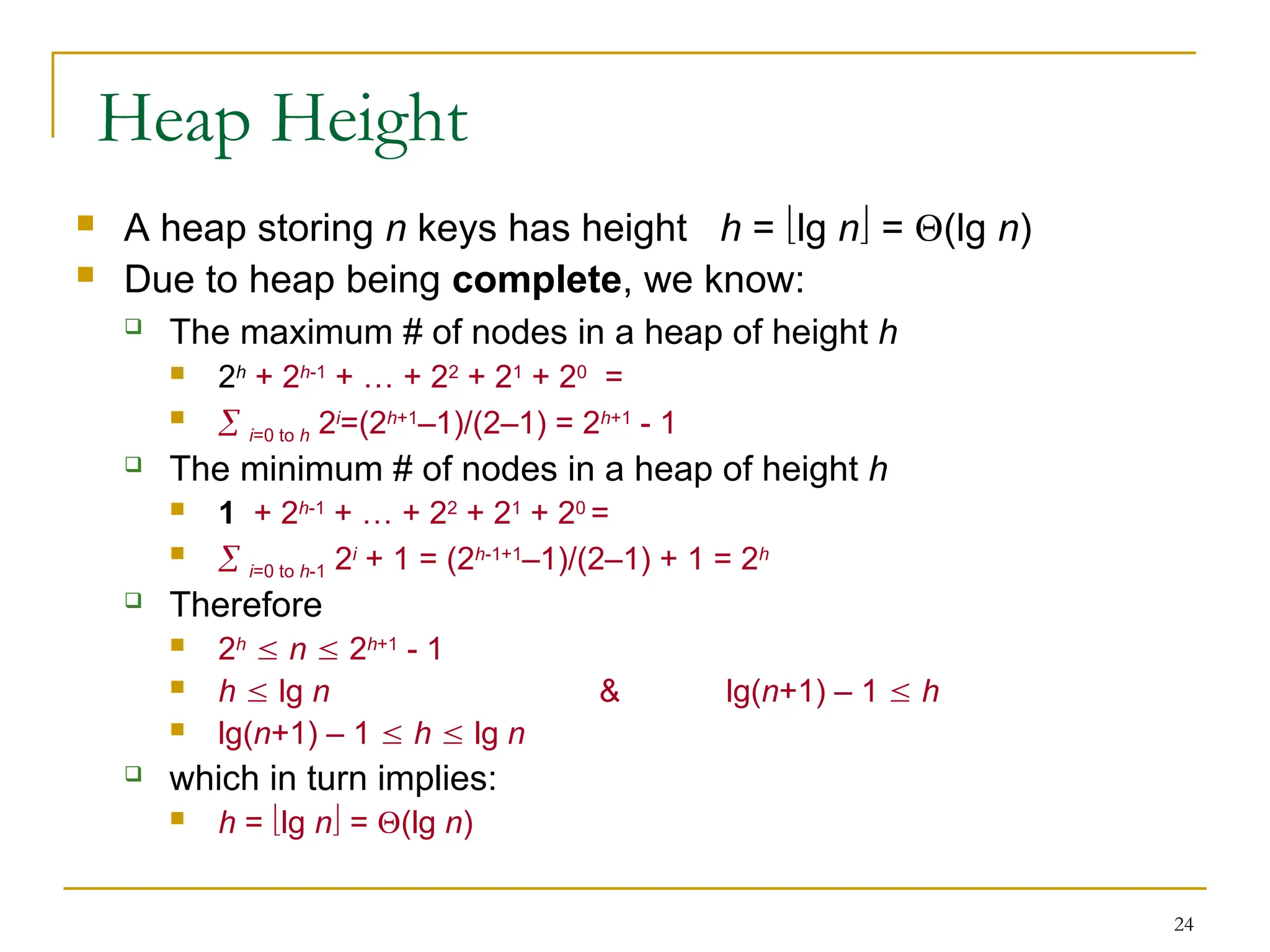
Heap Height
 A heap storing n keys has height h = lg n = (lg n)
 Due to heap being complete, we know:
 The maximum # of nodes in a heap of height h
 2h
+ 2h-1
+ … + 22
+ 21
+ 20
=
  i=0 to h 2i
=(2h+1
–1)/(2–1) = 2h+1
- 1
 The minimum # of nodes in a heap of height h
 1 + 2h-1
+ … + 22
+ 21
+ 20
=
  i=0 to h-1 2i
+ 1 = (2h-1+1
–1)/(2–1) + 1 = 2h
 Therefore
 2h
 n  2h+1
- 1
 h  lg n & lg(n+1) – 1  h
 lg(n+1) – 1  h  lg n
 which in turn implies:
 h = lg n = (lg n)

22. 26
Analyzing Heapify
)(
 The running time at any given node i is
 (1) time to fix up the relationships among A[i],
A[Left(i)] and A[Right(i)]
 plus the time to call Heapify recursively on a sub-
tree rooted at one of the children of node I
 And, the children’s subtrees each have size
at most 2n/3

23. 27
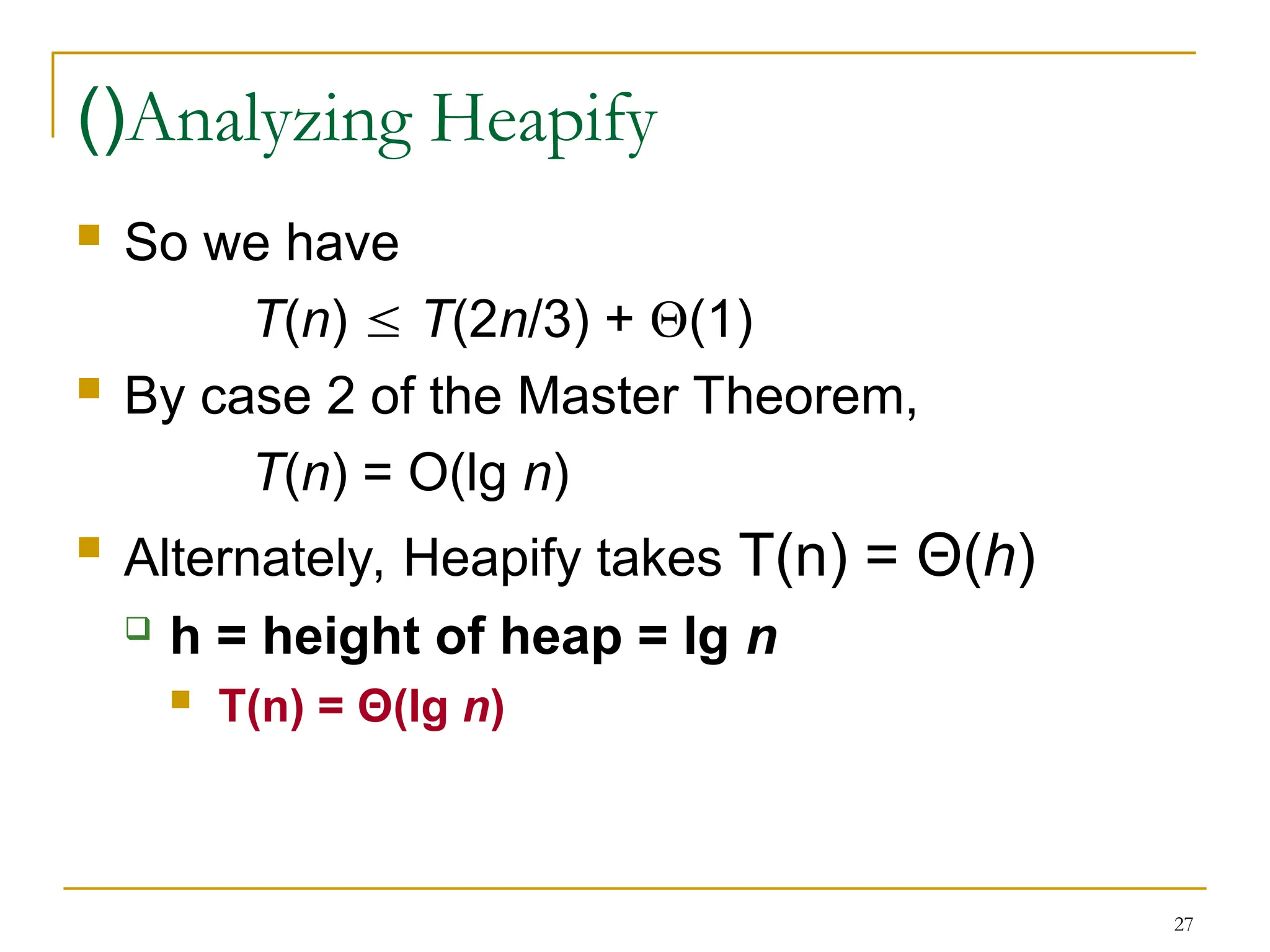
Analyzing Heapify
)(
 So we have
T(n)  T(2n/3) + (1)
 By case 2 of the Master Theorem,
T(n) = O(lg n)
 Alternately, Heapify takes T(n) = Θ(h)
 h = height of heap = lg n
 T(n) = Θ(lg n)

24. 28
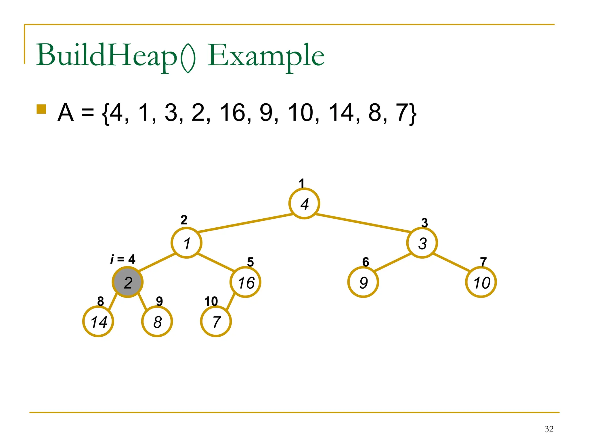
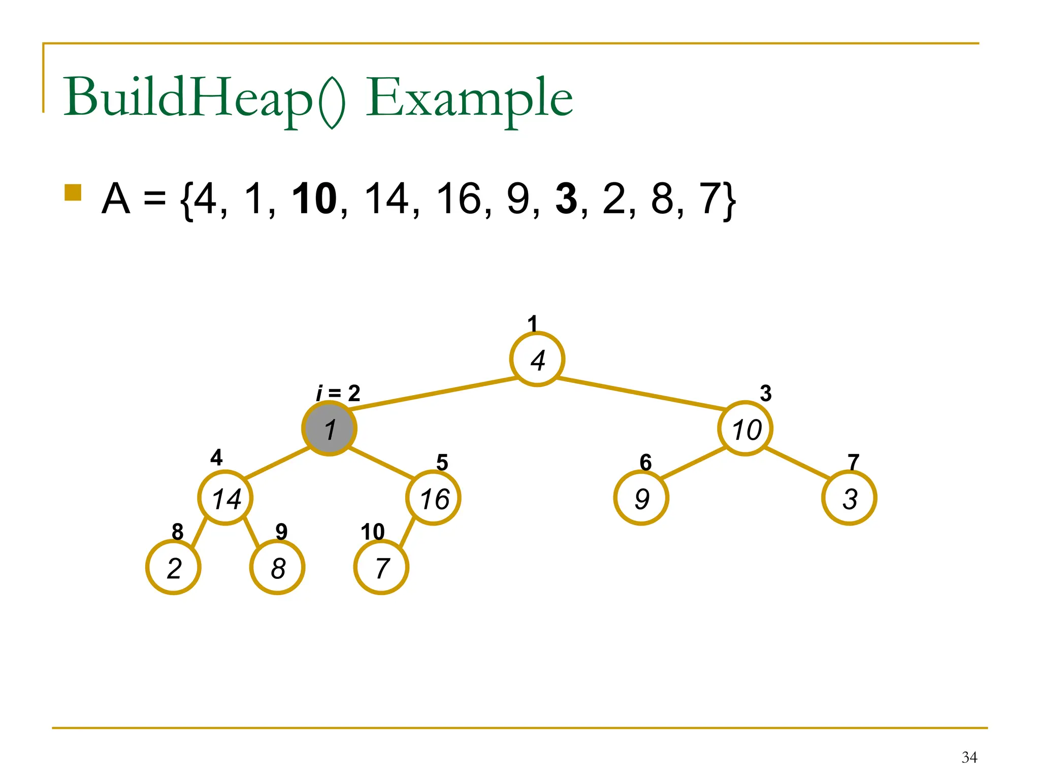
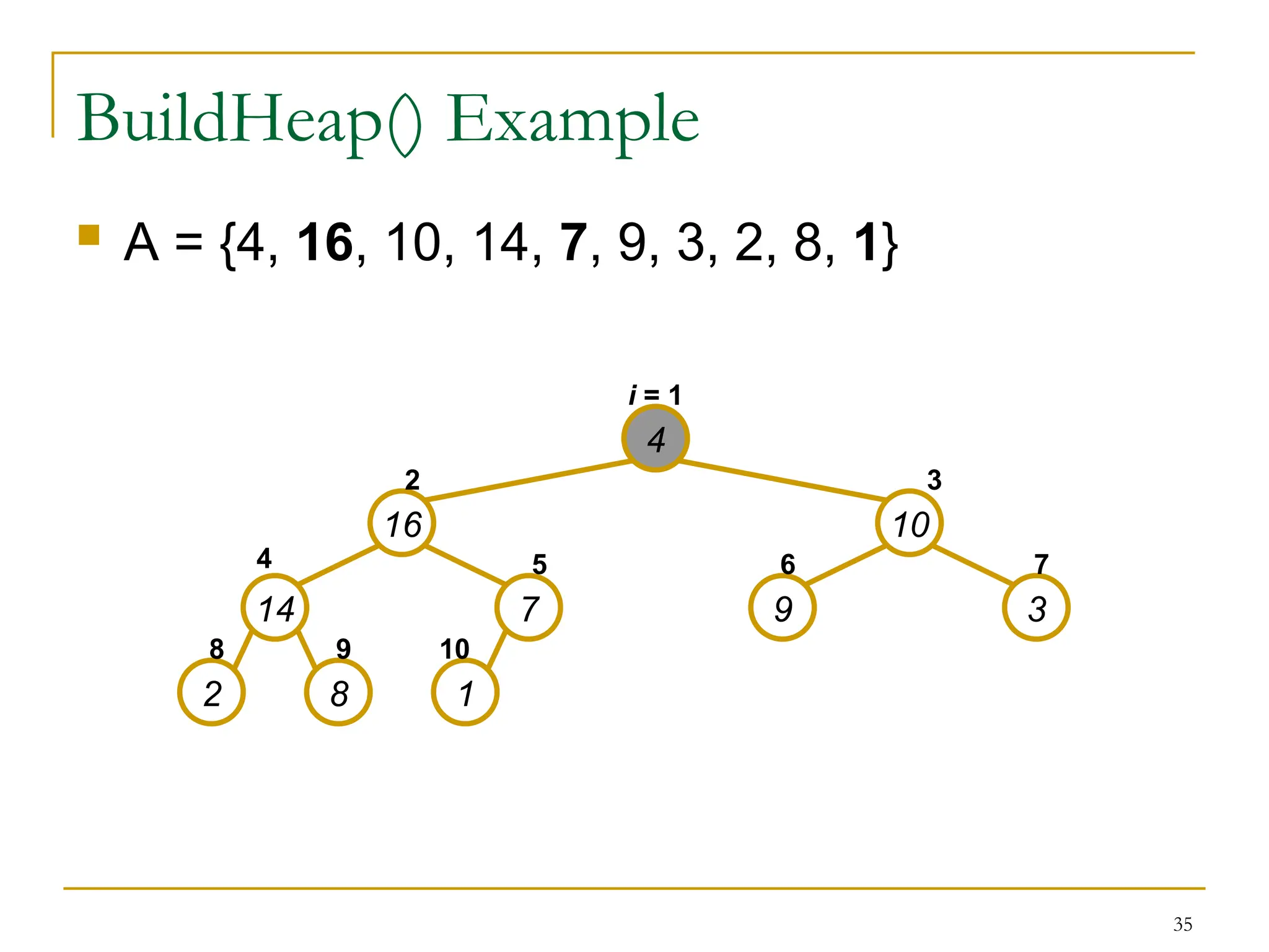
Heap Operations: BuildHeap
)(
 We can build a heap in a bottom-up manner by
running Heapify() on successive subarrays
 Fact: for array of length n, all elements in range
A[n/2 + 1, n/2 + 2 .. n] are heaps (Why?)
 These elements are leaves, they do not have children
 We also know that the leave-level has at most 2h
nodes = n/2 nodes
 and other levels have a total of n/2 nodes
 Walk backwards through the array from n/2 to
1, calling Heapify() on each node.

25. 29
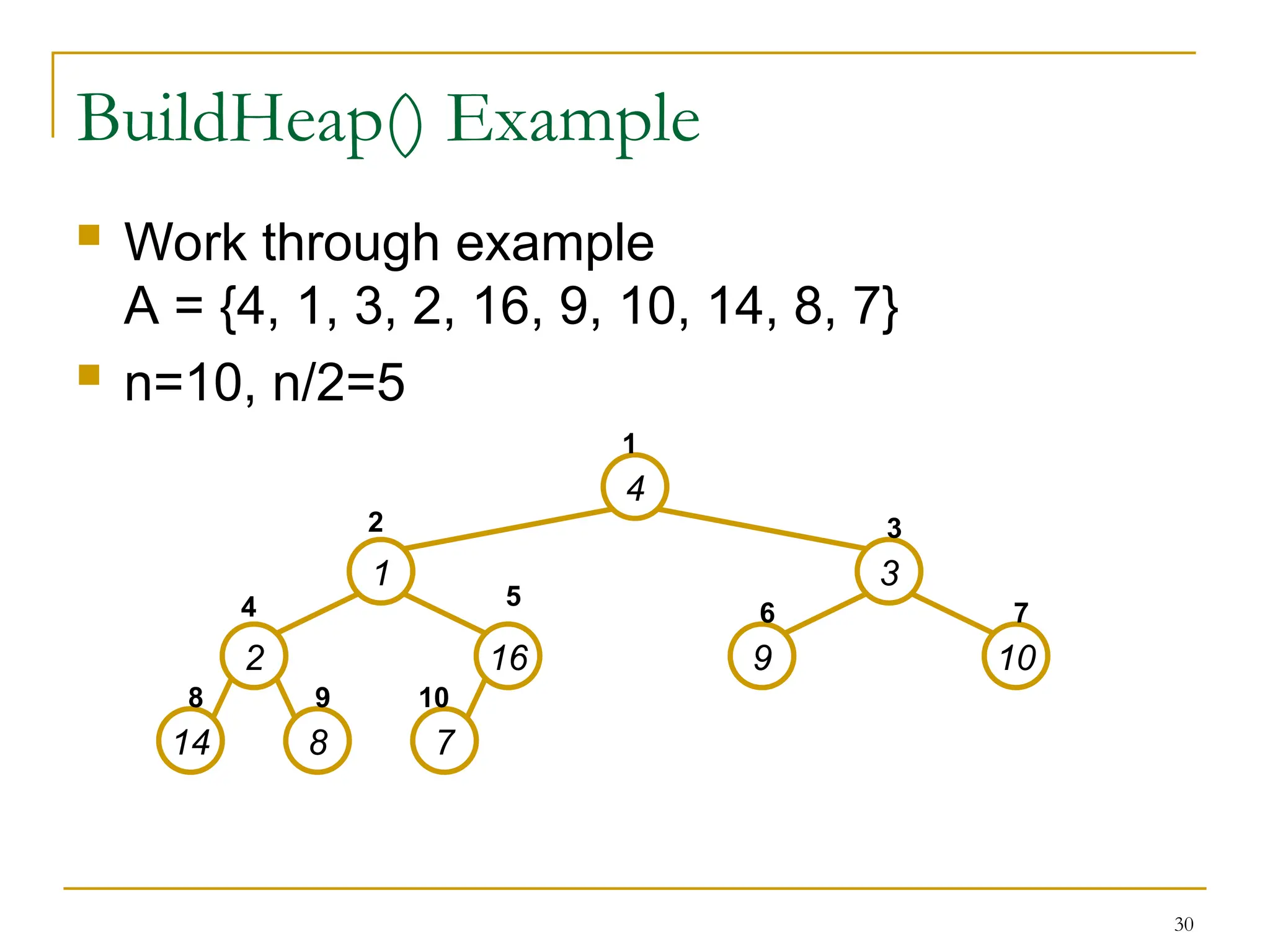
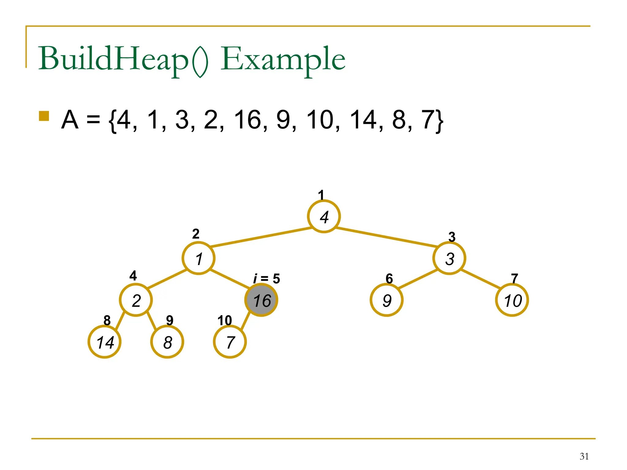
BuildHeap
)(
// given an unsorted array A, make A a heap
BuildHeap(A)
{
1. heap-size[A]  length[A]
2. for i  length[A]/2 downto 1
3. do Heapify(A, i)
}
 The Build Heap procedure, which runs in linear time,
produces a max-heap from an unsorted input array.
 However, the Heapify procedure, which runs in
O(lg n) time, is the key to maintaining the heap property.

26. 30
BuildHeap() Example
 Work through example
A = {4, 1, 3, 2, 16, 9, 10, 14, 8, 7}
 n=10, n/2=5
4
1 3
2 16 9 10
14 8 7
1
2 3
4 5
6 7
8 9 10

27. 31
BuildHeap() Example
 A = {4, 1, 3, 2, 16, 9, 10, 14, 8, 7}
4
1 3
2 16 9 10
14 8 7
1
2 3
4 i = 5 6 7
8 9 10

28. 32
BuildHeap() Example
 A = {4, 1, 3, 2, 16, 9, 10, 14, 8, 7}
4
1 3
2 16 9 10
14 8 7
1
2 3
i = 4 5 6 7
8 9 10

29. 33
BuildHeap() Example
 A = {4, 1, 3, 14, 16, 9, 10, 2, 8, 7}
4
1 3
14 16 9 10
2 8 7
1
2 i = 3
4 5 6 7
8 9 10

30. 34
BuildHeap() Example
 A = {4, 1, 10, 14, 16, 9, 3, 2, 8, 7}
4
1 10
14 16 9 3
2 8 7
1
i = 2 3
4 5 6 7
8 9 10

31. 35
BuildHeap() Example
 A = {4, 16, 10, 14, 7, 9, 3, 2, 8, 1}
4
16 10
14 7 9 3
2 8 1
i = 1
2 3
4 5 6 7
8 9 10

32. 36
BuildHeap() Example
 A = {16, 14, 10, 8, 7, 9, 3, 2, 4, 1}
16
14 10
8 7 9 3
2 4 1
1
2 3
4 5 6 7
8 9 10

33. 37
Analyzing BuildHeap
)(
 Each call to Heapify() takes O(lg n) time
 There are O(n) such calls (specifically, n/2)
 Thus the running time is O(n lg n)
 Is this a correct asymptotic upper bound?
 YES
 Is this an asymptotically tight bound?
 NO
 A tighter bound is O(n)
 How can this be? Is there a flaw in the above reasoning?
 We can derive a tighter bound by observing that the time for
Heapify to run at a node varies with the height of the node in
the tree, and the heights of most nodes are small.
 Fact: an n-element heap has at most 2h-k
nodes of
level k, where h is the height of the tree.

34. 38
Analyzing BuildHeap(): Tight
 The time required by Heapify on a node of height k is O(k). So
we can express the total cost of BuildHeap as
k=0 to h 2h-k
O(k) = O(2h
k=0 to h k/2k
)
= O(n k=0 to h k(½)k
)
From: k=0 to ∞ k xk
= x/(1-x)2
where x =1/2
So, k=0 to  k/2k
= (1/2)/(1 - 1/2)2
= 2
Therefore, O(n k=0 to h k/2k
) = O(n)
 So, we can bound the running time for building a heap from
an unordered array in linear time

35. 39
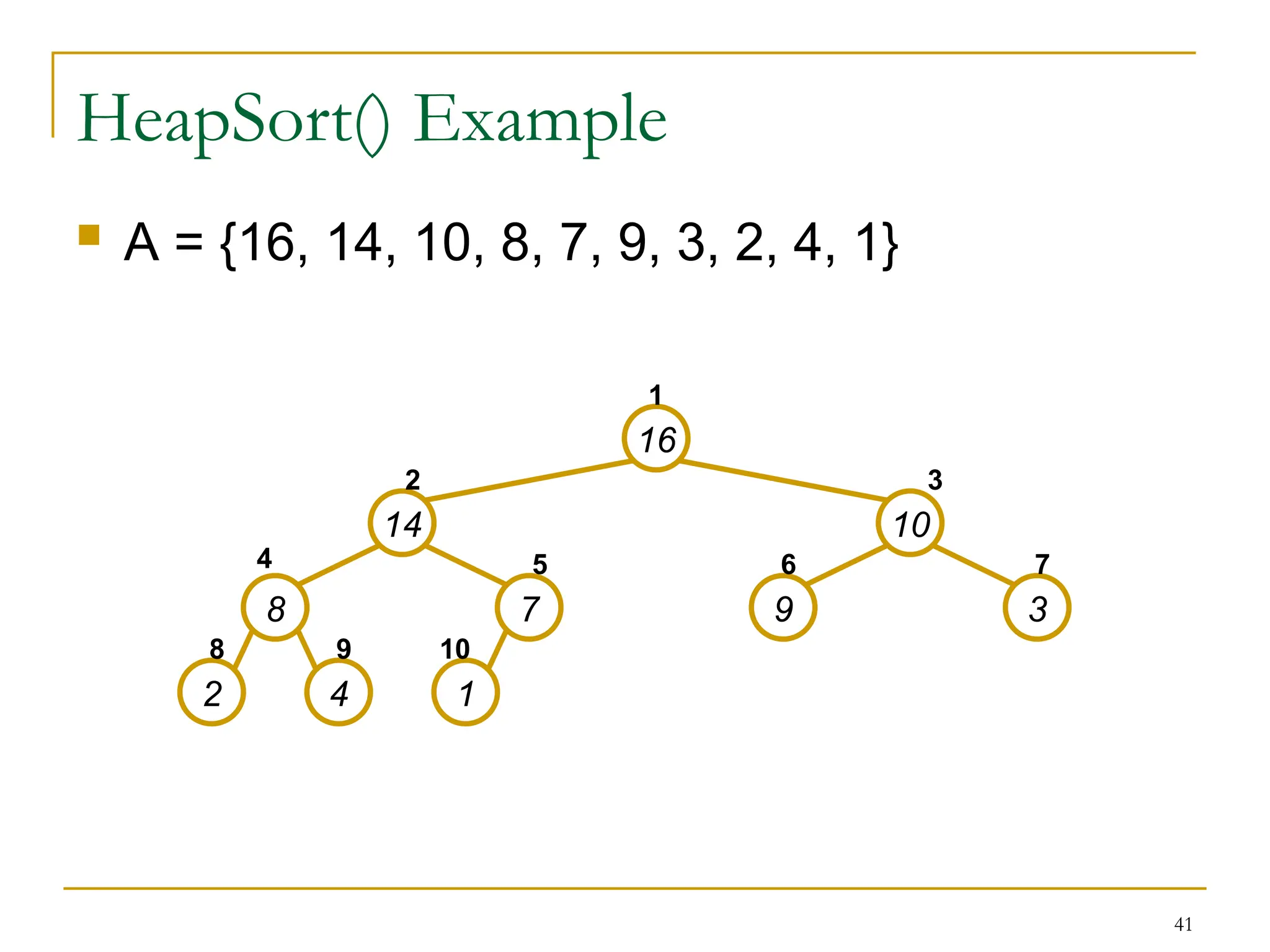
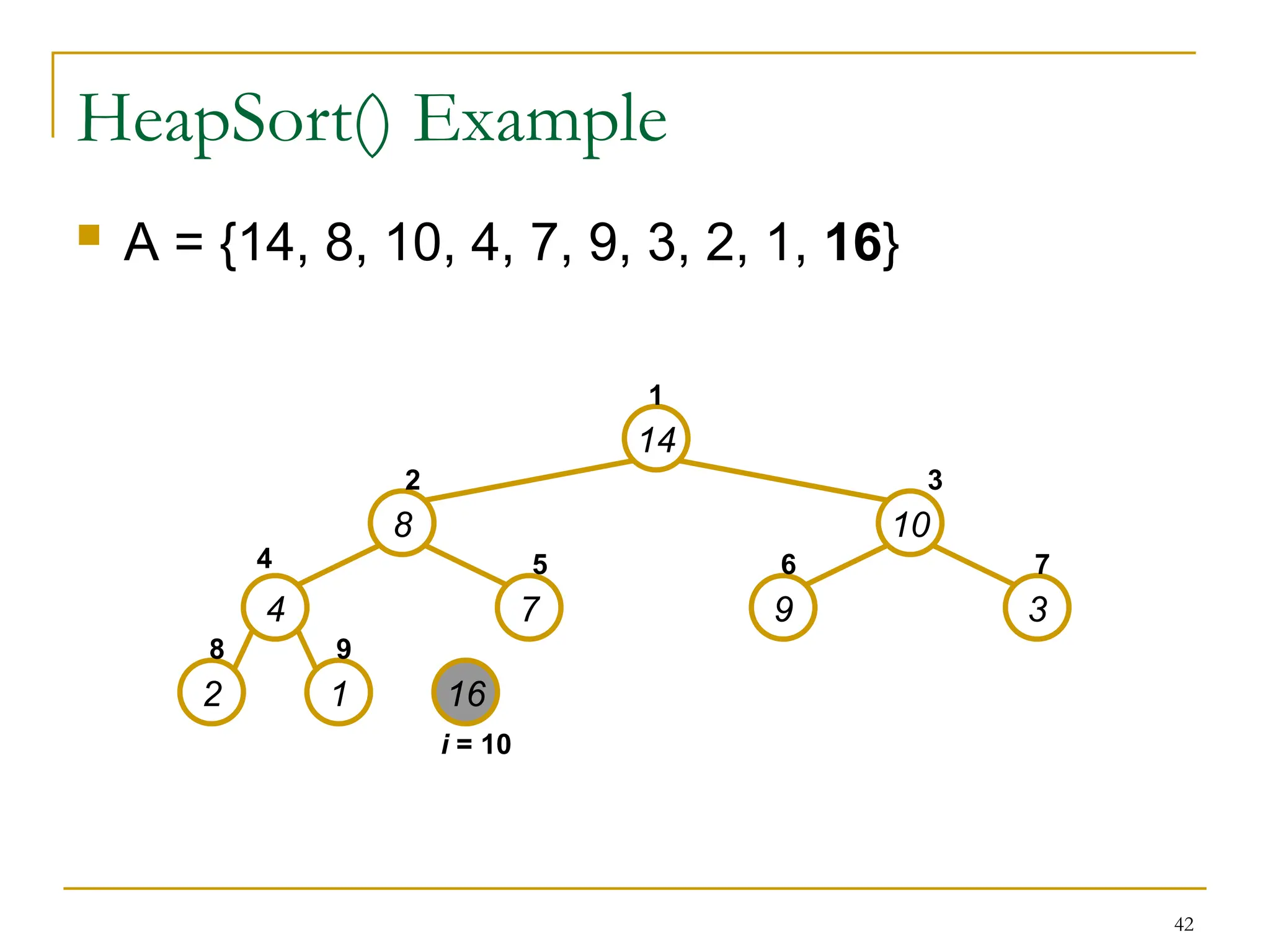
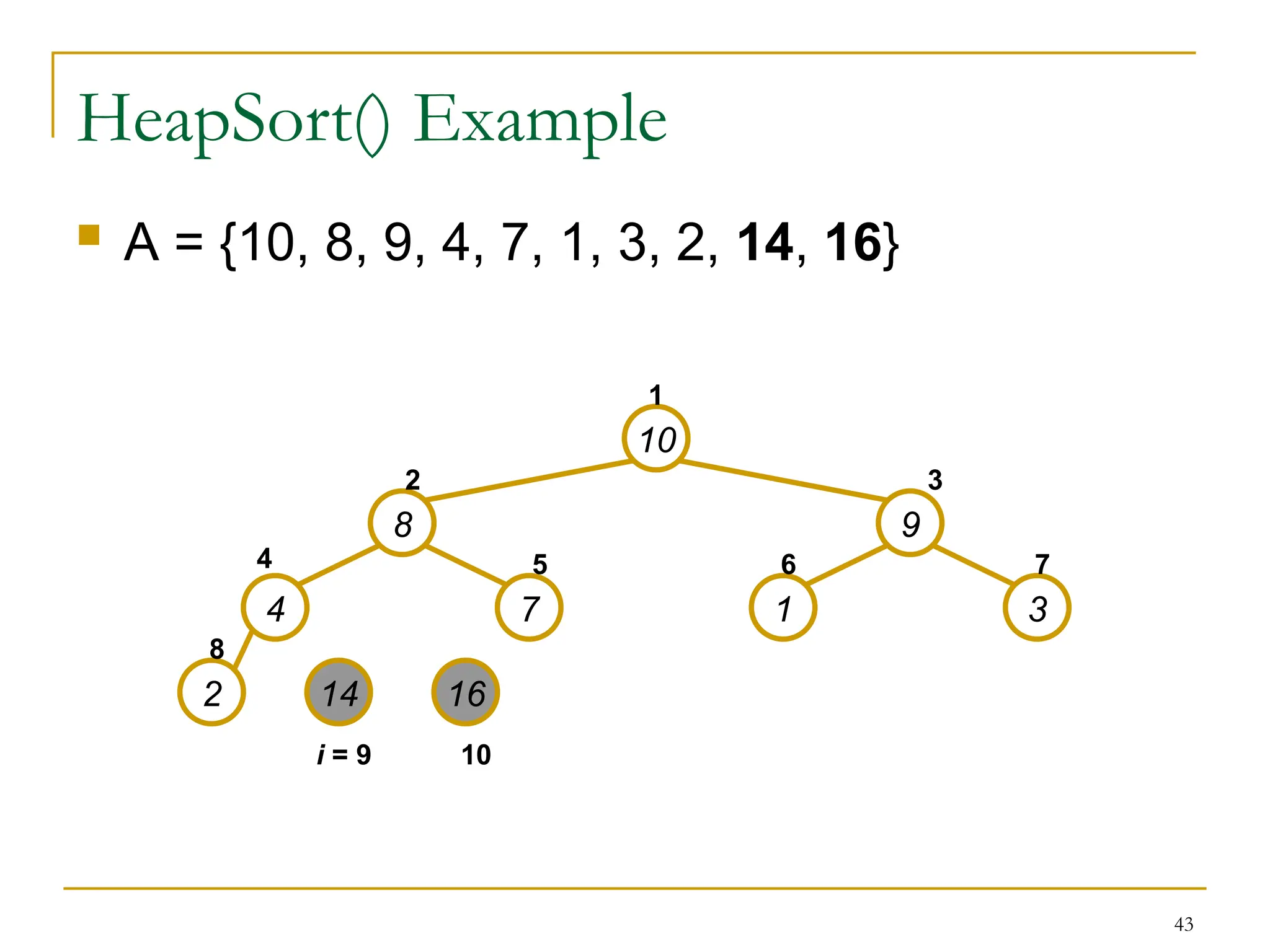
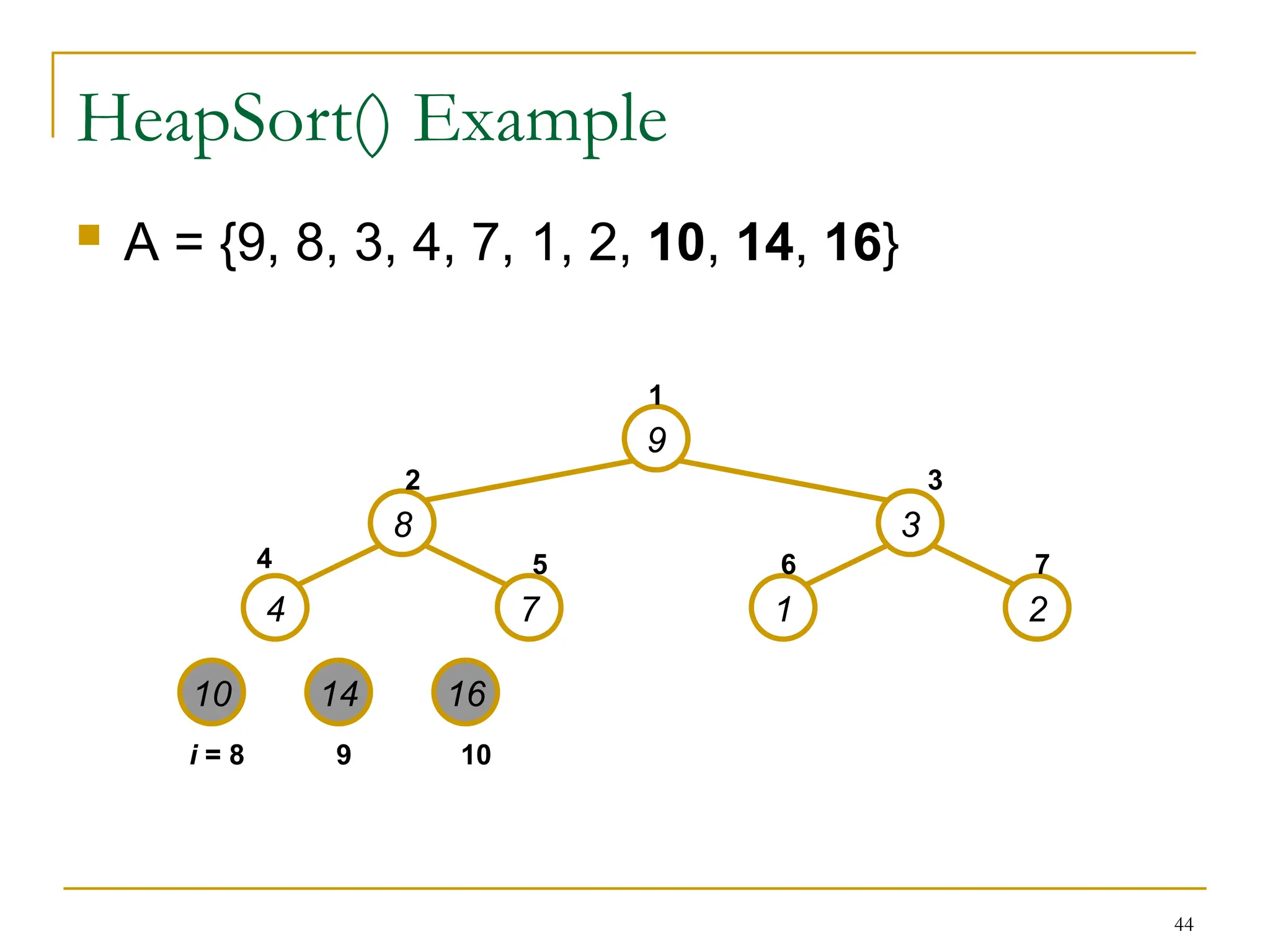
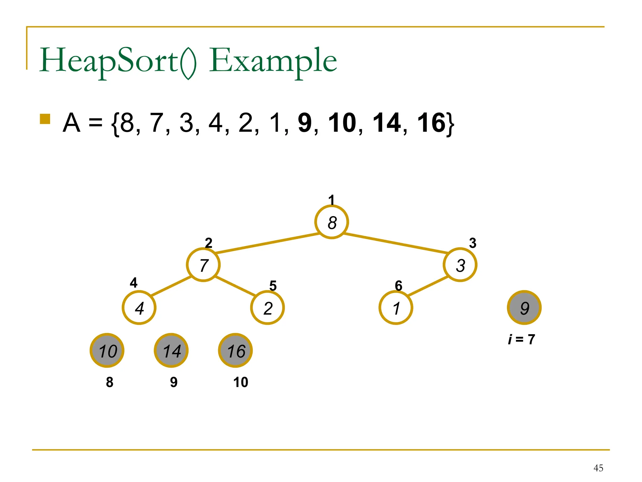
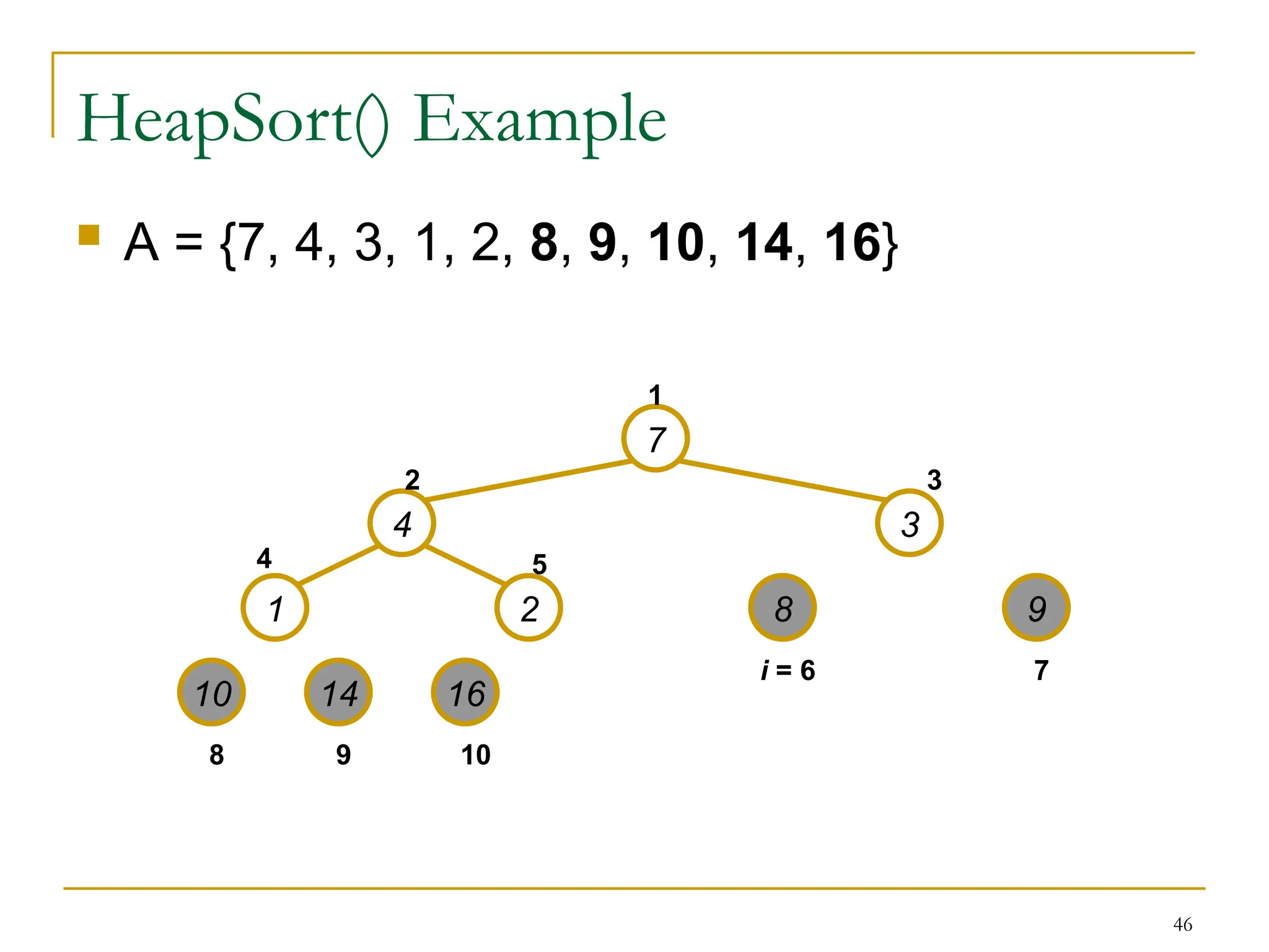
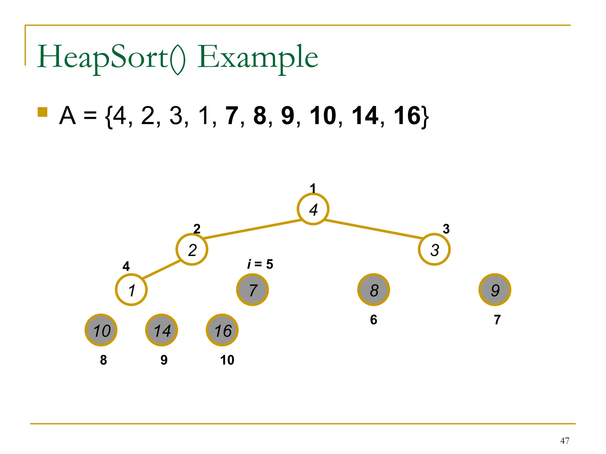
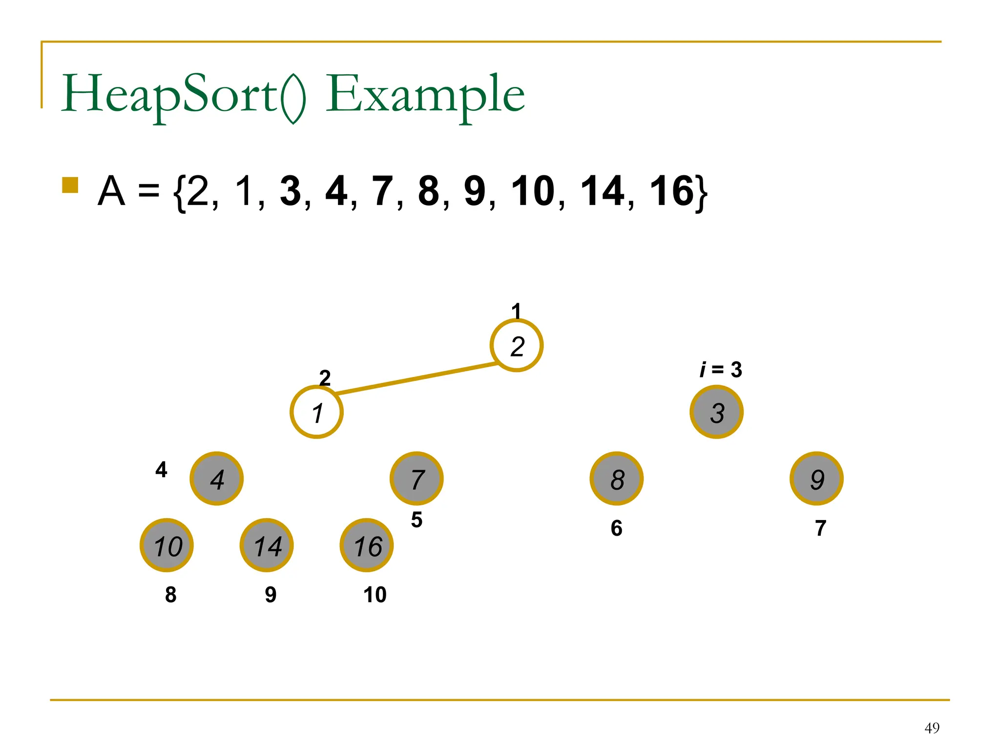
Heapsort
 Given BuildHeap(), an in-place sorting
algorithm is easily constructed:
 Maximum element is at A[1]
 Discard by swapping with element at A[n]
 Decrement heap_size[A]
 A[n] now contains correct value
 Restore heap property at A[1] by calling
Heapify()
 Repeat, always swapping A[1] for
A[heap_size(A)]

36. 40
Heapsort
Heapsort(A)
{
1. Build-Heap(A)
2. for i  length[A] downto 2
3. do exchange A[1]  A[i]
4. heap-size[A]  heap-size[A] - 1
5. Heapify(A, 1)
}

37. 41
HeapSort() Example
 A = {16, 14, 10, 8, 7, 9, 3, 2, 4, 1}
16
14 10
8 7 9 3
2 4 1
1
2 3
4 5 6 7
8 9 10

38. 42
HeapSort() Example
 A = {14, 8, 10, 4, 7, 9, 3, 2, 1, 16}
14
8 10
4 7 9 3
2 1 16
1
2 3
4 5 6 7
8 9
i = 10

39. 43
HeapSort() Example
 A = {10, 8, 9, 4, 7, 1, 3, 2, 14, 16}
10
8 9
4 7 1 3
2 14 16
1
2 3
4 5 6 7
8
10
i = 9

40. 44
HeapSort() Example
 A = {9, 8, 3, 4, 7, 1, 2, 10, 14, 16}
9
8 3
4 7 1 2
10 14 16
1
2 3
4 5 6 7
9 10
i = 8

41. 45
HeapSort() Example
 A = {8, 7, 3, 4, 2, 1, 9, 10, 14, 16}
8
7 3
4 2 1 9
10 14 16
1
2 3
4 5 6
8 9 10
i = 7

42. 46
HeapSort() Example
 A = {7, 4, 3, 1, 2, 8, 9, 10, 14, 16}
7
4 3
1 2 8 9
10 14 16
1
2 3
4 5
7
8 9 10
i = 6

43. 47
HeapSort() Example
 A = {4, 2, 3, 1, 7, 8, 9, 10, 14, 16}
4
2 3
1 7 8 9
10 14 16
1
2 3
4
6 7
8 9 10
i = 5

44. 48
HeapSort() Example
 A = {3, 2, 1, 4, 7, 8, 9, 10, 14, 16}
3
2 1
4 7 8 9
10 14 16
1
2 3
5 6 7
8 9 10
i = 4

45. 49
HeapSort() Example
 A = {2, 1, 3, 4, 7, 8, 9, 10, 14, 16}
2
1 3
4 7 8 9
10 14 16
1
2
4
5 6 7
8 9 10
i = 3

46. 50
HeapSort() Example
 A = {1, 2, 3, 4, 7, 8, 9, 10, 14, 16}
1
2 3
4 7 8 9
10 14 16
1
3
4
5 6 7
8 9 10
i =2

47. 51
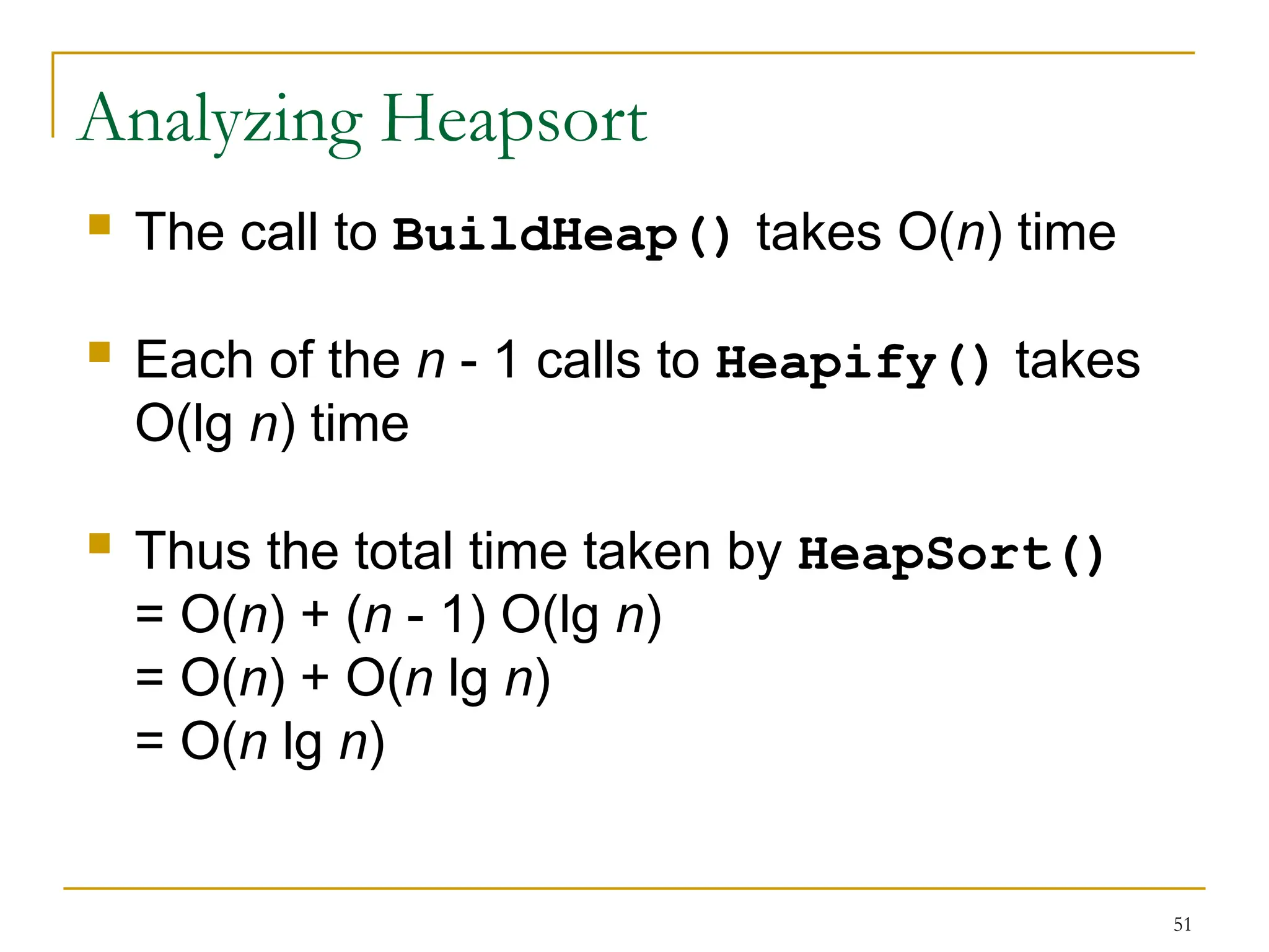
Analyzing Heapsort
 The call to BuildHeap() takes O(n) time
 Each of the n - 1 calls to Heapify() takes
O(lg n) time
 Thus the total time taken by HeapSort()
= O(n) + (n - 1) O(lg n)
= O(n) + O(n lg n)
= O(n lg n)

48. 52
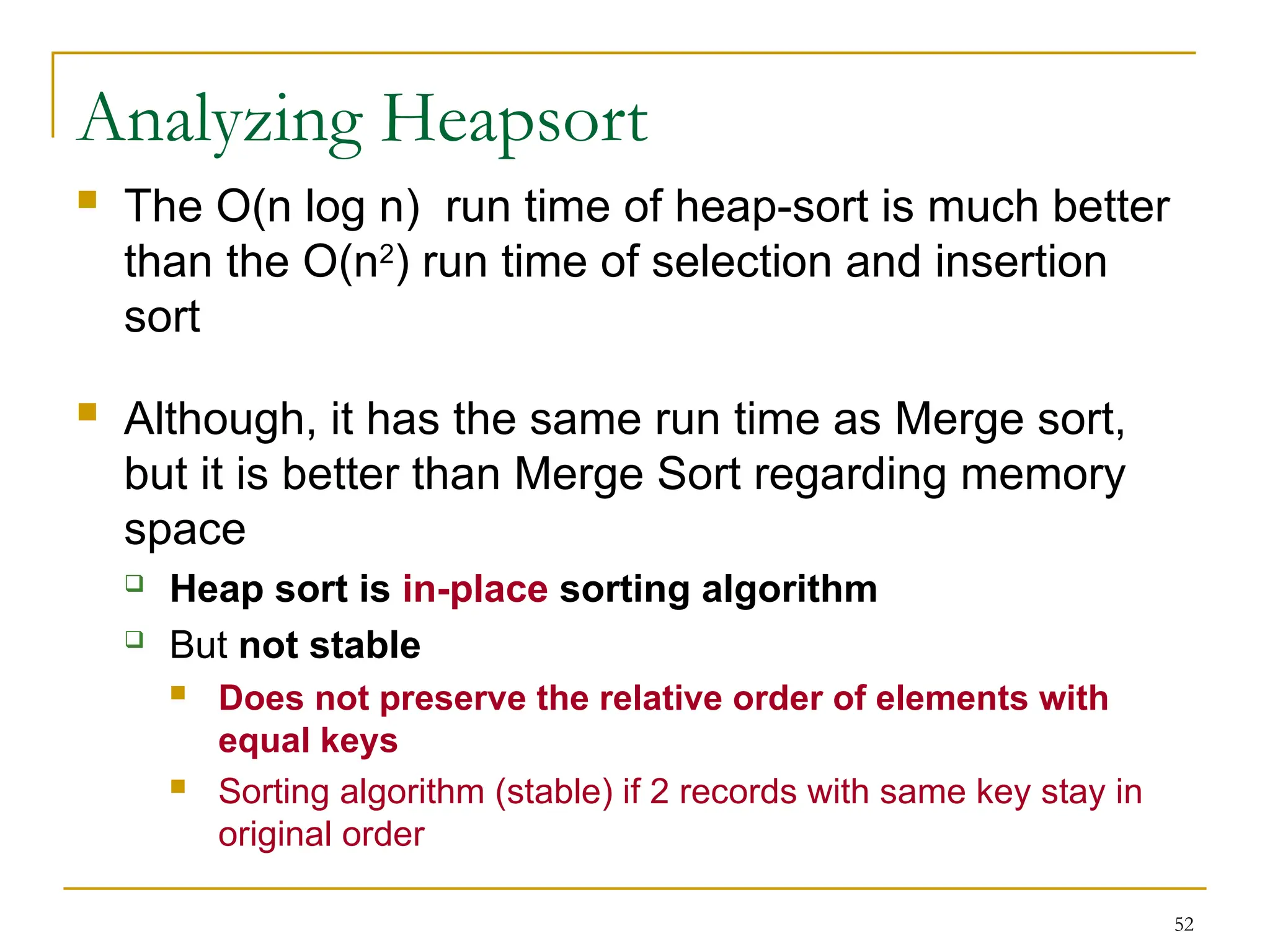
Analyzing Heapsort
 The O(n log n) run time of heap-sort is much better
than the O(n2
) run time of selection and insertion
sort
 Although, it has the same run time as Merge sort,
but it is better than Merge Sort regarding memory
space
 Heap sort is in-place sorting algorithm
 But not stable
 Does not preserve the relative order of elements with
equal keys
 Sorting algorithm (stable) if 2 records with same key stay in
original order

49. 53
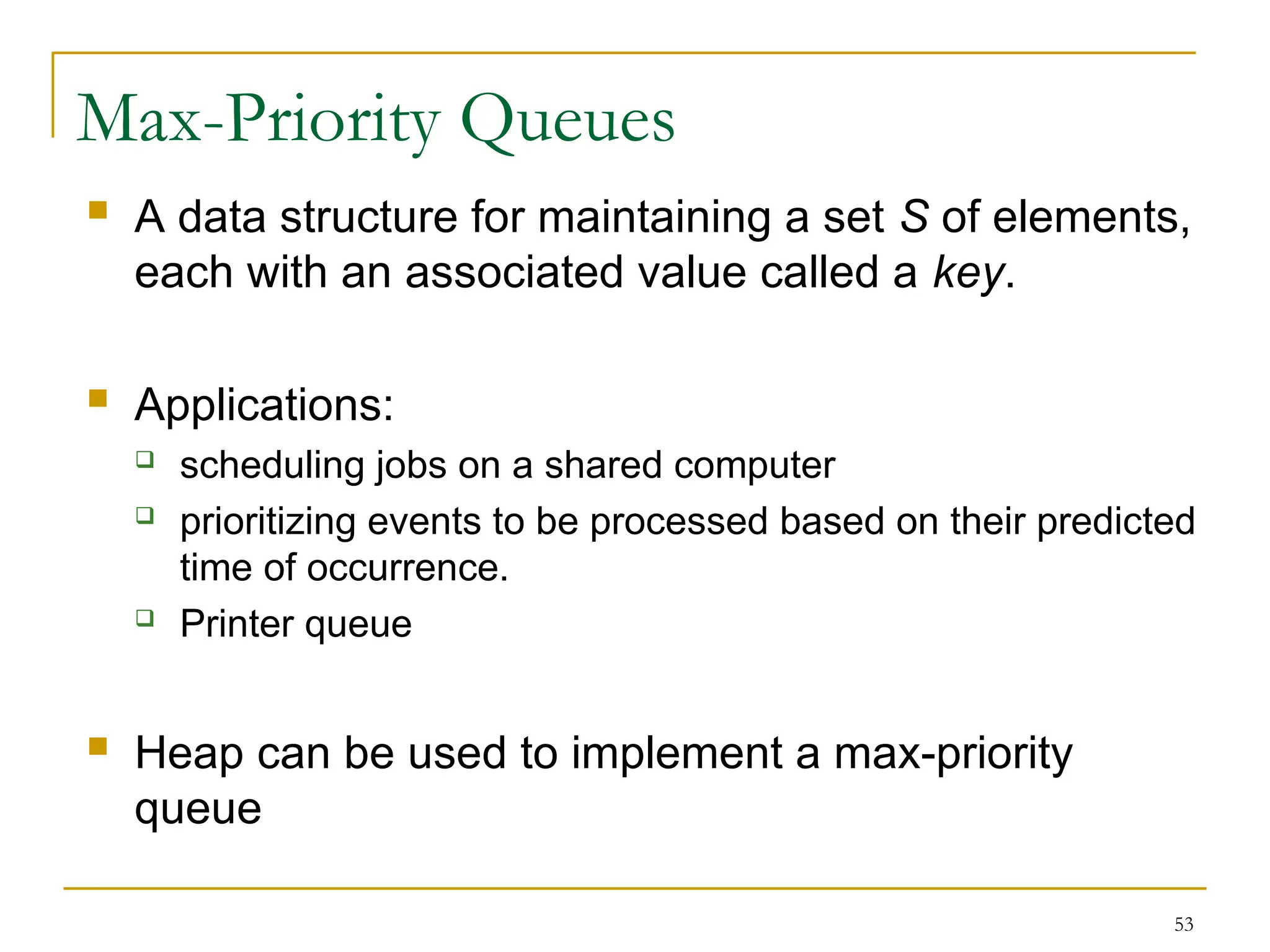
Max-Priority Queues
 A data structure for maintaining a set S of elements,
each with an associated value called a key.
 Applications:
 scheduling jobs on a shared computer
 prioritizing events to be processed based on their predicted
time of occurrence.
 Printer queue
 Heap can be used to implement a max-priority
queue

50. 54
Max-Priority Queue: Basic Operations
 Maximum(S): return A[1]
 returns the element of S with the largest key (value)
 Extract-Max(S):
 removes and returns the element of S with the largest key
 Increase-Key(S, x, k):
 increases the value of element x’s key to the new value k,
x.value  k
 Insert(S, x):
 inserts the element x into the set S, i.e. S  S  {x}

51. 55
Extract-Max(A)
1. if heap-size[A] < 1 // zero elements
2. then error “heap underflow”
3. max  A[1]// max element in first position
4. A[1]  A[heap-size[A]]
// value of last position assigned to first position
5. heap-size[A]  heap-size[A] – 1
6. Heapify(A, 1)
7. return max
Note lines 3-5 are similar to the for loop
body of Heapsort procedure

52. 56
Increase-Key(A, i, key)
// increase a value (key) in the array
1. if key < A[i]
2. then error “new key is smaller than current key”
3. A[i]  key
4. while i > 1 and A[Parent(i)] < A[i]
5. do exchange A[i]  A[Parent(i)]
6. i  Parent(i) // move index up to parent

53. 57
Increase-Key() Example
 A = {16, 14, 10, 8, 7, 9, 3, 2, 4, 1}
16
14 10
8 7 9 3
2 4 1
1
2 3
4 5 6 7
8 i=9 10

54. 58
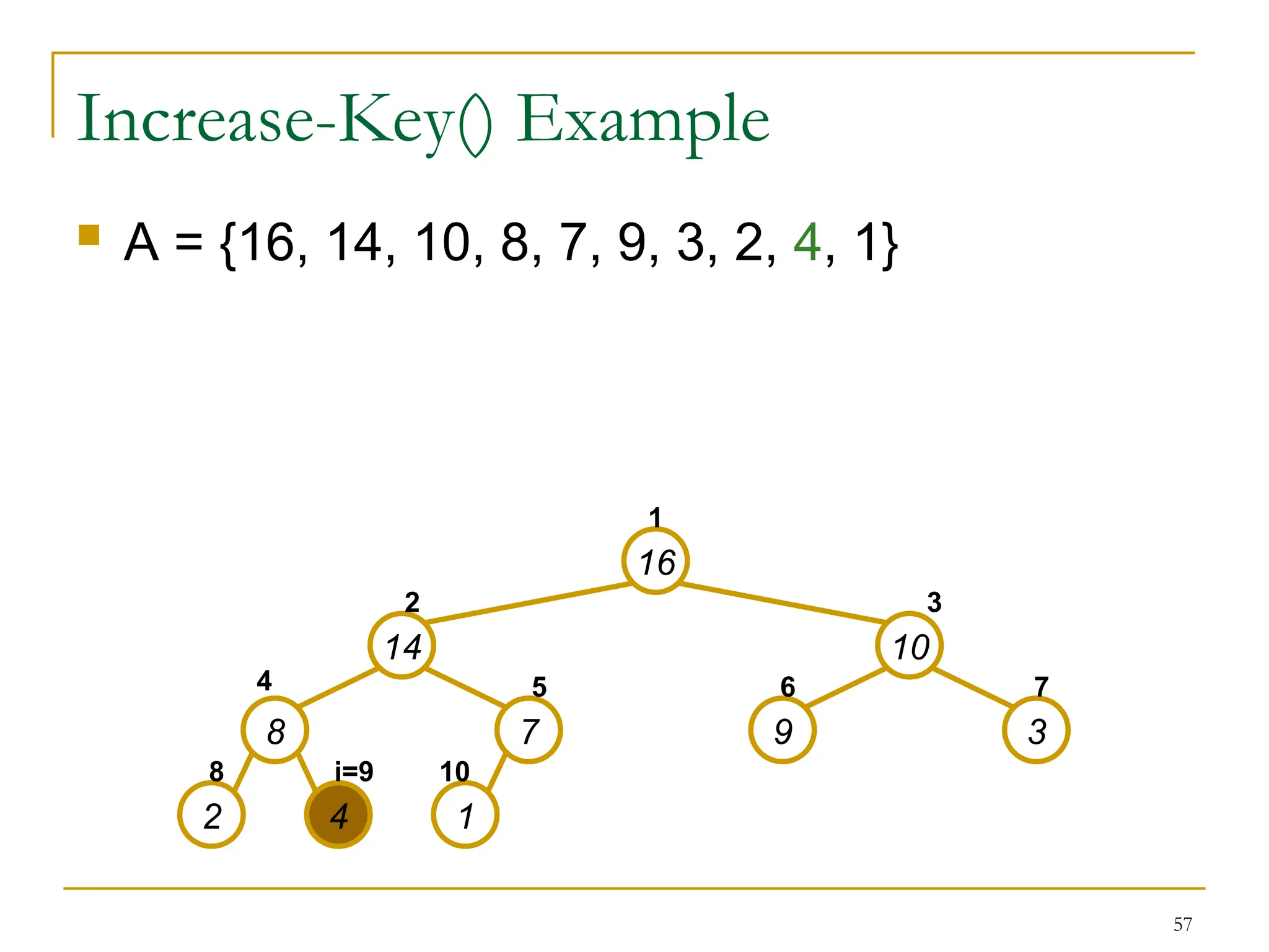
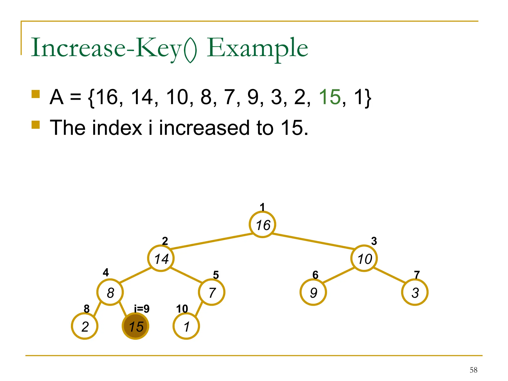
Increase-Key() Example
 A = {16, 14, 10, 8, 7, 9, 3, 2, 15, 1}
 The index i increased to 15.
16
14 10
8 7 9 3
2 15 1
1
2 3
4 5 6 7
8 i=9 10

55. 59
Increase-Key() Example
 A = {16, 14, 10, 15, 7, 9, 3, 2, 8, 1}
 After one iteration of the while loop of lines 4-
6, the node and its parent have exchanged
keys (values), and the index i moves up to
the parent.
16
14 10
15 7 9 3
2 8 1
1
2 3
i=4 5 6 7
8 9 10

56. 60
Increase-Key() Example
 A = {16, 15, 10, 14, 7, 9, 3, 2, 8, 1}
 After one more iteration of the while loop.
 The max-heap property now holds and the
procedure terminates.
16
15 10
14 7 9 3
2 8 1
1
2 3
i=4 5 6 7
8 9 10

57. 61
Insert(A, key)
// insert a value at the end of the binary tree
then move it in the right position
1. heap-size[A]  heap-size[A] + 1
2. A[heap-size[A]]  -
3. Increase-Key(A, heap-size[A], key)

58. 62
Example: Operation of Heap Insert

59. 63
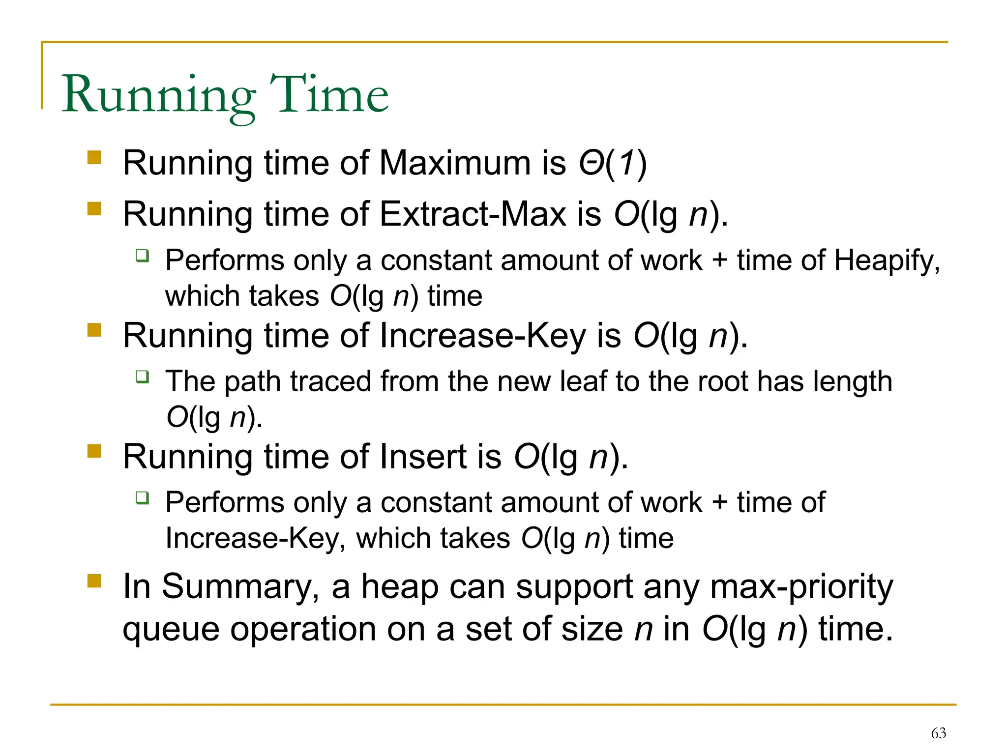
Running Time
 Running time of Maximum is Θ(1)
 Running time of Extract-Max is O(lg n).
 Performs only a constant amount of work + time of Heapify,
which takes O(lg n) time
 Running time of Increase-Key is O(lg n).
 The path traced from the new leaf to the root has length
O(lg n).
 Running time of Insert is O(lg n).
 Performs only a constant amount of work + time of
Increase-Key, which takes O(lg n) time
 In Summary, a heap can support any max-priority
queue operation on a set of size n in O(lg n) time.