This document describes the heap data structure and its implementation using arrays. It discusses binary heaps, including max heap and min heap properties. It covers heap operations like insertion, deletion, building a heap, extracting the max/min, and getting the max/min. Heapsort is also summarized, which uses a heap to sort elements in O(n log n) time without extra space.

1. Heap
Data Structure
Abdur Rouf
1505097
Aditya Chakma
1505120
Course Teacher :
Madhusudan Basak
Mahmudur Rahman Hera
Department of Computer Science and Engineering
Bangladesh University of Engineering and Technology
(BUET)
Dhaka 1000

2. Contents
0.1 Introduction . . . . . . . . . . . . . . . . . . . . . . . . . . . . . . 2
0.1.1 What is the Heap data structure? . . . . . . . . . . . . . 2
0.1.2 Application of Heap . . . . . . . . . . . . . . . . . . . . . 2
0.2 Variants of Heap . . . . . . . . . . . . . . . . . . . . . . . . . . . 3
0.3 Binary Heap Properties . . . . . . . . . . . . . . . . . . . . . . . 4
0.3.1 Max Heap Properties . . . . . . . . . . . . . . . . . . . . 5
0.3.2 Min Heap Properties . . . . . . . . . . . . . . . . . . . . . 5
0.4 Heap Implementation Using Arrays . . . . . . . . . . . . . . . . . 5
0.5 Binary heap Operation . . . . . . . . . . . . . . . . . . . . . . . . 6
0.5.1 Heap Insertion . . . . . . . . . . . . . . . . . . . . . . . . 7
0.5.2 Heap Deletion . . . . . . . . . . . . . . . . . . . . . . . . 10
0.5.3 Build Heap . . . . . . . . . . . . . . . . . . . . . . . . . . 12
0.5.4 Extract Max . . . . . . . . . . . . . . . . . . . . . . . . . 13
0.5.5 Get Max . . . . . . . . . . . . . . . . . . . . . . . . . . . 16
0.5.6 Heap Sort . . . . . . . . . . . . . . . . . . . . . . . . . . . 17
0.6 Heap Sort Analysis . . . . . . . . . . . . . . . . . . . . . . . . . . 21
0.7 Conclusion . . . . . . . . . . . . . . . . . . . . . . . . . . . . . . 21
1

3. 0.1 Introduction
The heap data structure is a very useful data structure.We will be going through
a brief introduction on the heap data structure.Like most data structures, the
heap data structure is often labelled as an advanced topic. One that only the
computer science majors, and the brave dare to learn and understand. As we
unravel the contents, you will hopefully begin to realize that it is not as difficult
as you once thought.This writings will not be tied down to a specific language.
In another words, regardless of what programming language you use, you will
be able to follow, understand and benefit from this writings.Understanding the
heap data structure will make you more complete as a programmer.
0.1.1 What is the Heap data structure?
A heap is a specialized tree-based data structure that satisfied the heap property:
If C is a child node of P, then key(P) ≥ key(C). This implies that an element
with the greatest key is always in the root node, and so such a heap is sometimes
called a max-heap. Of course, there’s also a min-heap.
P
C C
Figure 1: Heap
0.1.2 Application of Heap
The heap is a very useful data structure. Some popular algorithms such as the
heap sort use the heap data structure behind the scenes. Other use cases include
• Finding the min, max, median value in a collection of data.
• Graph algorithms
• priority queues. The heap is a concrete implementation of the priority
queue abstract data type.
• Schedulers (for finding the first/earliest action item on the schedule).
• Dijkstra’s shortest path algorithm.
2

4. 0.2 Variants of Heap
There are many type of heaps such as
• Fibonacci Heap
• 2-3 Heap
• Binary heap
• etc
In this report we will discuss on binary heap, it’s implementation and also time
complexity elaborately
3

5. 0.3 Binary Heap Properties
Below are some of the features of the heap data structures
• Both left and right child of node may be smaller(max heap) or greater(min
heap) simultaneously.
• For each level of the tree, the data is inserted from left to right.
• A new level of the tree is NOT started until the current level is filled from
left to right.
Let me use the example below to clarify.
As you can see in figure:2, unlike in the binary search tree, the left Child is
not necessarily lesser than the right child. As long as the parent is greater than
its children, it a valid heap.
If we were to insert another node into the heap below, it will be inserted as
a left child of node with key of 5.
The tree currently has a depth of four. Level four will continue to be filled
and a new level will not be started until the node with key value 1 (index 6)
has both a left and a right child.
0
1 2
3 4
7 8
5 6
80
18
40
13 5
25 1
2 9
0 1 2 3 4 5 6 7 8
1880 40 13 5 25 1 2 9
Figure 2: Tree and Array Representation of Heap
Figure:2 refers max heap actually. But it may two types.
• Max Heap
• Min Heap
Now we discuss on max heap and min heap properties.
4

6. 0.3.1 Max Heap Properties
Lets take a look at the properties that define the max heap.
• The key of parent nodes are greater than or equal to (>=) that of the
children.
• Therefore, the highest key is at the root node.
0.3.2 Min Heap Properties
To put things into perspective, the min heap is the inverted result of the max
heap.
• The key of parent nodes are lower than or equal to (<=) that of the
children.
• Therefore, the lowest key is at the root node.
0.4 Heap Implementation Using Arrays
A complete binary tree can be uniquely represented by storing its level order
traversal in an array.
The root is the second item in the array. We skip the index zero cell of the array
for the convenience of implementation. Consider k−th element of the array, then
• its left child is located at 2 ∗ k index
• its right child is located at 2 ∗ k + 1 index
• its parent is located at k
2 index
Now we will introduce with Heapify Algorithm.As we discuss on Max
Heap which is discussed earlier, here we see max heapify algorithm. Basically
all heap operation is directly or indirectly use this heapify function. Here is the
Heapify Algorithm
5

7. MAX-HEAPIFY(A,i)
1 l ← left(i);
2 r ← right(i);
3 if l ≤ heapsize[A]andA[l] > A[i] then
4 largest ← l;
5 end
6 else
7 largest ← i;
8 end
9 if r ≤ heapsize[A]andA[r] > A[largest] then
10 largest ← r;
11 end
12 if largest = i then
13 exchangeA[i] ↔ A[largest];
14 MAX − HEAPIFY (A, largest);
15 end
0.5 Binary heap Operation
In this section, We will see 6 binary Heap operation one by one.
1. Heap Insertion
2. Heap Deletion
3. Build Heap
4. Extract Max
5. Get Max
6. Heap Sort
6

8. 0.5.1 Heap Insertion
Considering that, we have a prebuild heap. Then we insert 17 in this Heap.We
will discuss insertion by demonstration of tree structure of heap.
22
15 20
12 14 6 18
11 10
Insert 17
Here 17 will be inserted at the last of the heap array which actually the left
child of 14.
22
15 20
12 14 6 18
11 10
Insert 17
17 < 14 false
17
7

9. Here 17 is greater than 14. So 17 and 14 will be swapped. this operation
actually handled by Heapify Function
22
15 20
12 17 6 18
11 10
Insert 17
14
This tree isn’t heapified fully. Because still here 15 is less than 17 though 17
is the right child of 15 which violate max heap property.
22
15 20
12 17 6 18
11 10
Insert 17
17 < 15 false
14
8

10. In the previous way 17 and 15 will be swapped here. Here 17 is less than
22
17 20
12 15 6 18
11 10
Insert 17
14
22 and also 17 is child of 22. So, it’s fulfill the heap property. So after inserting
17, the final representation of the tree will be this type.
22
17 20
12 15 6 18
11 10
Insert 17
DONE!
17 < 22 true
14
9

11. Here is the algorithm for heap insertion
MAX-HEAP-INSERT(A,key)
1 heapsize[A] ← heapsize[A] + 1;
2 A[heapsize[A]] ← −∞;
3 A[i] ← key;
4 while i > 1 and A[parent(i)] < A[i] do
5 exchange A[i] ↔ A[parent(i)];
6 i ← parent(i)
7 end
0.5.2 Heap Deletion
To delete 20, first we have to search that node and then replace it with the last
element of the tree which is the left child of 15. Then deleting last element and
heapify the tree for preserving heap property.
22
17 20
12 15 6 18
11 10
Delete 20
14
10

12. in this figure 20 will be swapped with 14.
22
17 14
12 15 6 18
11 10
Delete 20
20
Now 20 wil be deleted and 14 will be compared with 22 and 18. As 22 is greater
so it will be unchanged but 14 is less than 18 which violate heap property.
22
17 14
12 15 6 18
11 10
Delete 20
22>14 true
but
14>18 false
11

13. Now So, 14 and 18 will be swapped and Heap Property again will be regained
22
17 18
12 15 6 14
11 10
Delete 20
DONE!
0.5.3 Build Heap
Build Heap is a function which has an array as an argument. And it returns a
heapified array which preserve all heap property.
BUILD-MAX-HEAP(A)
1 heapsize[A] ← lenght[A];
2 i ← length[A]
2 ;
3 while i ≥ 1 do
4 MAX − HEAPIFY (A, i);
5 i ← i − 1;
6 end
22
14
15 20
12 6 18
11 10
6 10 22 20 12 15 11 14 18
Build Heap
12

14. 0.5.4 Extract Max
Extract max actually the deletion of the root of the Max Heap.
Then we replace 22 with the last element of this heap which actually 10.
22
17 18
12 15 6 14
11 10
Extract max
10
17 18
12 15 6 14
11 22
Exchange 22 with last value
13

15. Now 22 will be removed.
10
17 18
12 15 6 14
11
Delete 22 and Heapify
Now 10 will be compared with 17 and 18. Here 18 is greater so 10 will be
replaced with 18.
18
17 10
12 15 6 14
11
still 10 is less than it’s child
14

16. Again 10 is compared with 14 and 6. As, 14 is greater so 10 will be replaced
with 14. Then we regain heap property. So, it’s done.
EXTRACT-MAX(A)
18
17 10
12 15 6 14
11
Here 14>6 so swap 10 with 14
18
17 14
12 15 6 10
11
DONE!
1 if heapsize[A] < 1 then
2 error”underflow”;
3 end
4 max ← A[1];
5 A[1] ← A[heapsize[A]];
6 heapsize[A] ← heapsize[A] − 1;
7 MAX − HEAPIFY (A, 1);
8 return max;
15

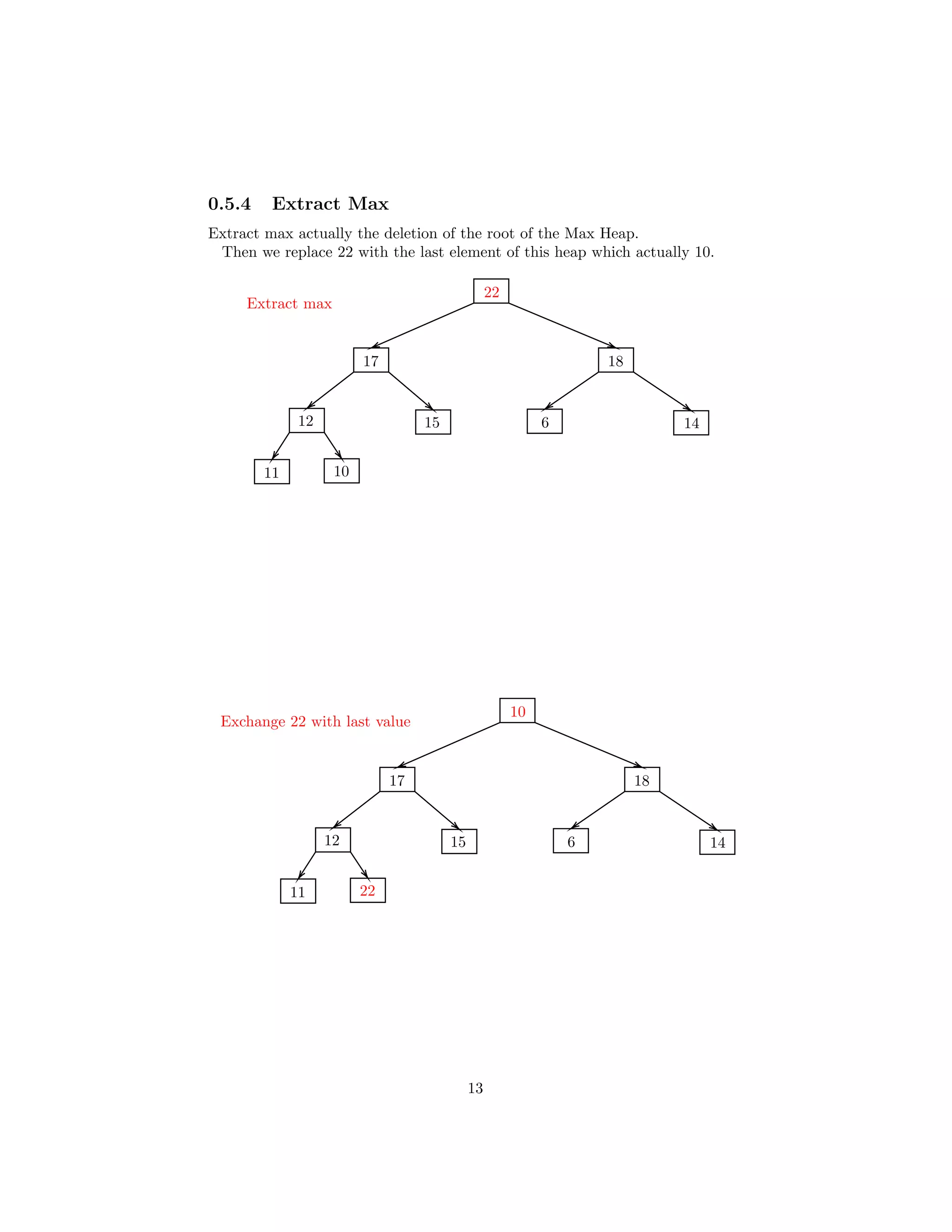
17. 0.5.5 Get Max
Get max function only reflect the root element value. It won’t delete the root.
18
17 14
12 15 6 10
11
Return root node value
18
17 14
12 15 6 10
11
max value = 18
HEAP-MAXIMUM(A)
1 return A[1];
16

18. 0.5.6 Heap Sort
Heap sort is a comparison based sorting technique based on Binary Heap data
structure. It is similar to selection sort where we first find the maximum element
and place the maximum element at the end. We repeat the same process for
remaining element.
18
17 14
12 15 6 10
11
Extract max
18
0 1 2 3 4 5 6 7
17
15 14
12 11 6 10
Extract max
18
0 1 2 3 4 5 6 7
17
17

19. 15
12 14
10 11 6
Extract max
18
0 1 2 3 4 5 6 7
17 15
14
12 6
10 11
Extract max
18
0 1 2 3 4 5 6 7
17 15 14
18

20. 12
11 6
10
Extract max
18
0 1 2 3 4 5 6 7
17 15 14 12
11
10 6
Extract max
18
0 1 2 3 4 5 6 7
17 15 14 12 11
19

21. 10
6
Extract max
18
0 1 2 3 4 5 6 7
17 15 14 12 11 10
6
Extract max
18
0 1 2 3 4 5 6 7
17 15 14 12 11 10 6
20

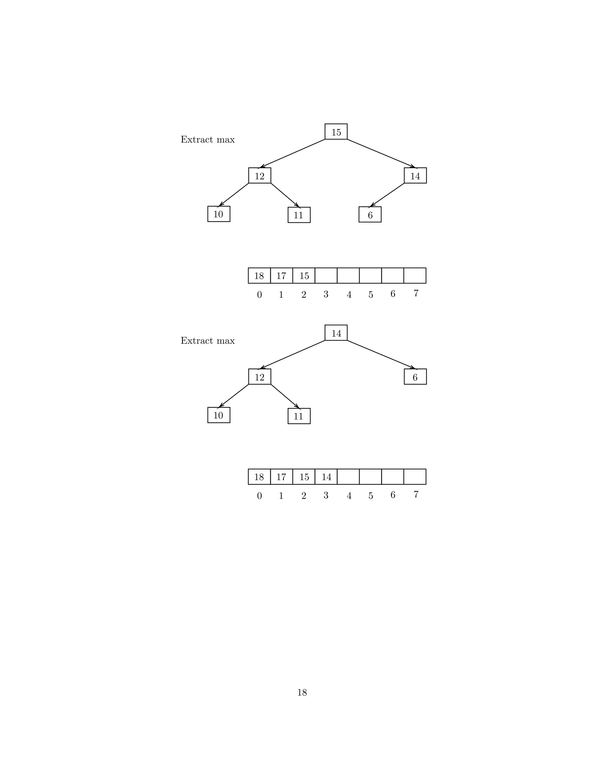
22. Here is the sorted array.
18
0 1 2 3 4 5 6 7
17 15 14 12 11 10 6
Sorted Array
The Algorithm for heap sort is given below
HEAP-SORT(A)
1 BUILD − HEAP(A);
2 i ← length[A];
3 while i ≥ 2 do
4 Swap(a[1], A[i]);
5 heapsize[A] ← heapsize[A] − 1;
6 i ← i − 1;
7 MAX − HEAPIFY (A, 1);
8 end
0.6 Heap Sort Analysis
• The call to BuildHeap() takes O(n) time
• Each of the n − 1 calls to Heapify() takes O(log n) time
• Thus the total time taken by HeapSort()
= O(n) + (n − 1)O(log n)
= O(n) + O(n log n)
= O(n log n)
0.7 Conclusion
With its time complexity of O(nlog(n)) heapsort is optimal. Unlike mergesort,
heapsort requires no extra space. On the other hand, heapsort is not stable. A
sorting algorithm is stable, if it leaves the order of equal elements unchanged.
The heap data structure can also be used for an efficient implementation of
a priority queue. A priority queue is an abstract list data structure with the
operations insert and extractMax. With each element in the list a certain prior-
ity is associated. By insert an element together with its priority is inserted into
the list. By extractMax the element with the highest priority is extracted from
the list. Using a heap, both operations can be implemented in time O(log(n)).
21