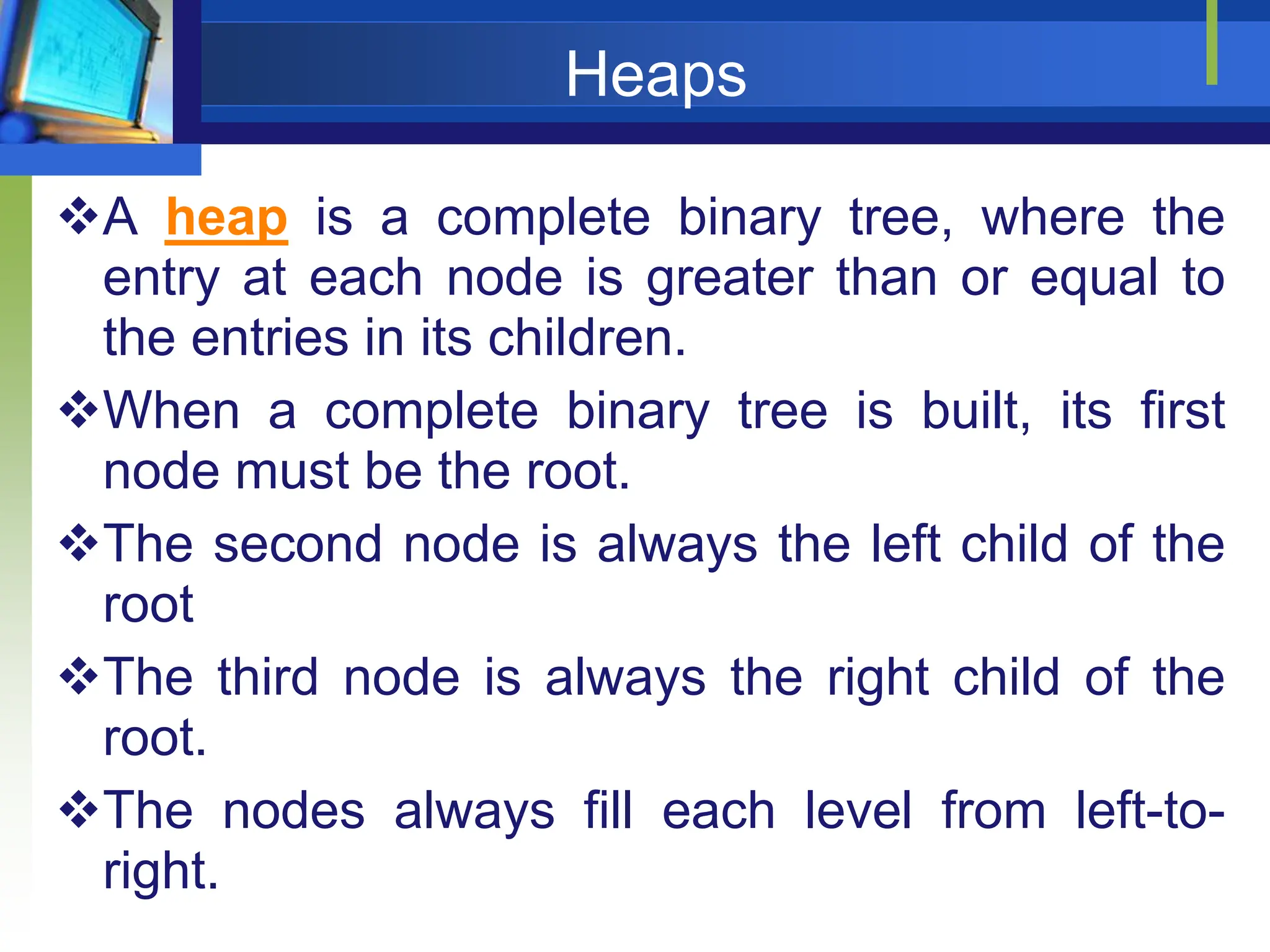
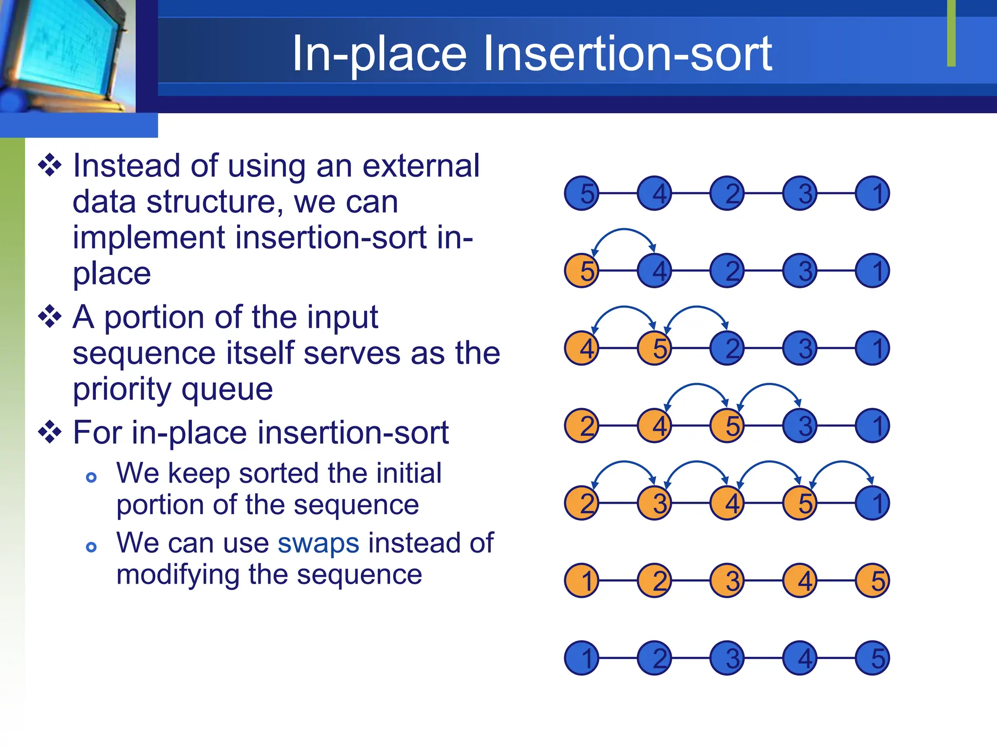
This document provides an overview of algorithms related to the design and analysis of recursive algorithms, specifically focusing on the master theorem and its applications. It also covers the concepts of heaps, heap sort, priority queues, and their implementations, including performance analysis and advantages. Key operations of priority queues and sorting techniques, particularly insertion sort, are discussed in detail.

![Definition
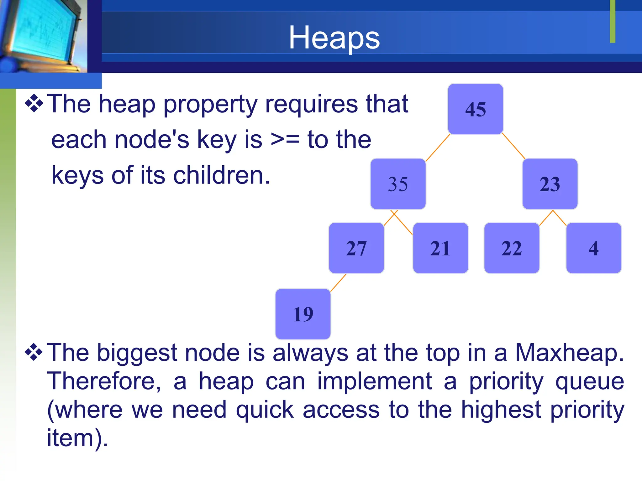
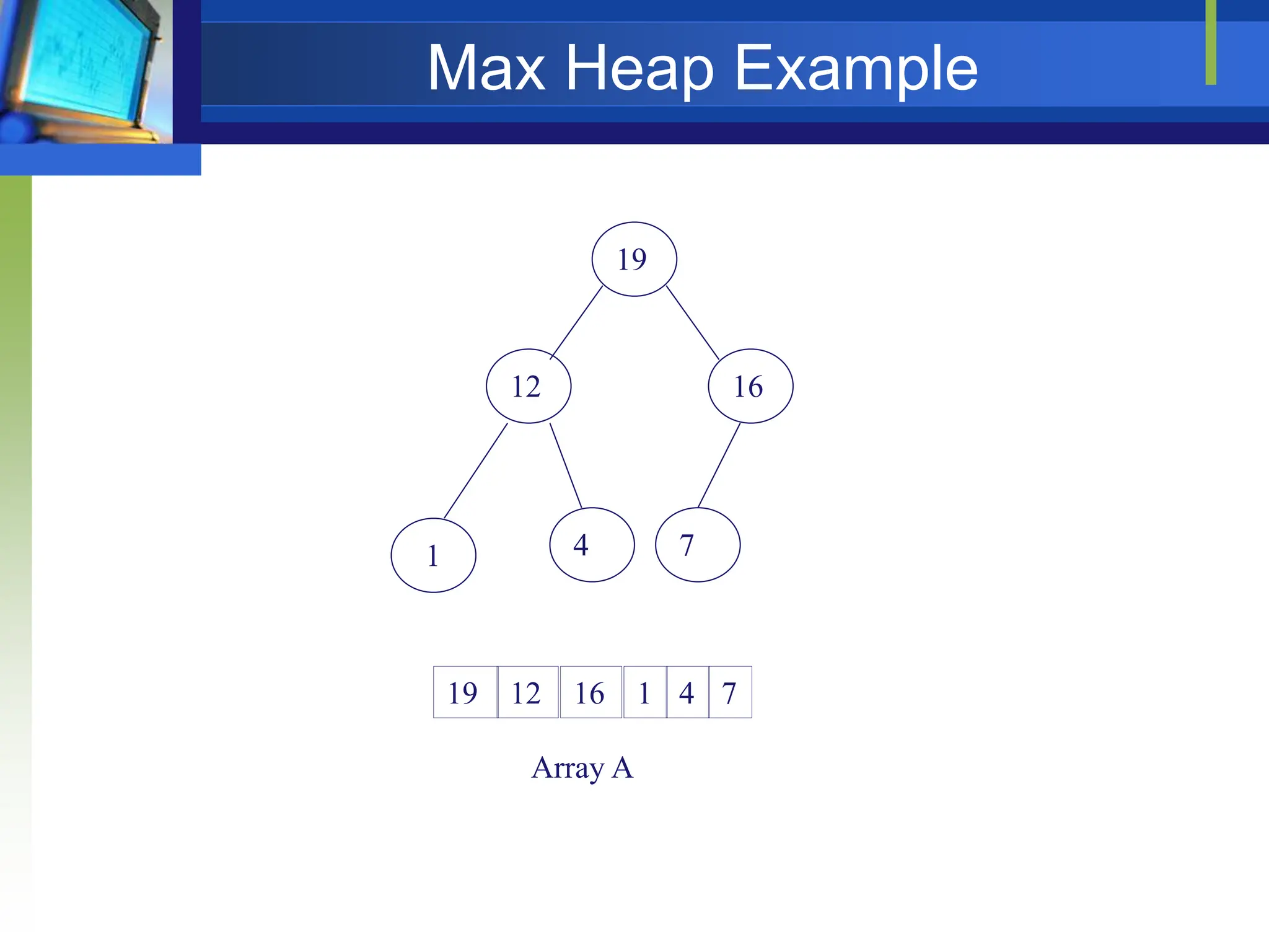
Max Heap
Store data in ascending order
Has property of
A[Parent(i)] ≥ A[i]
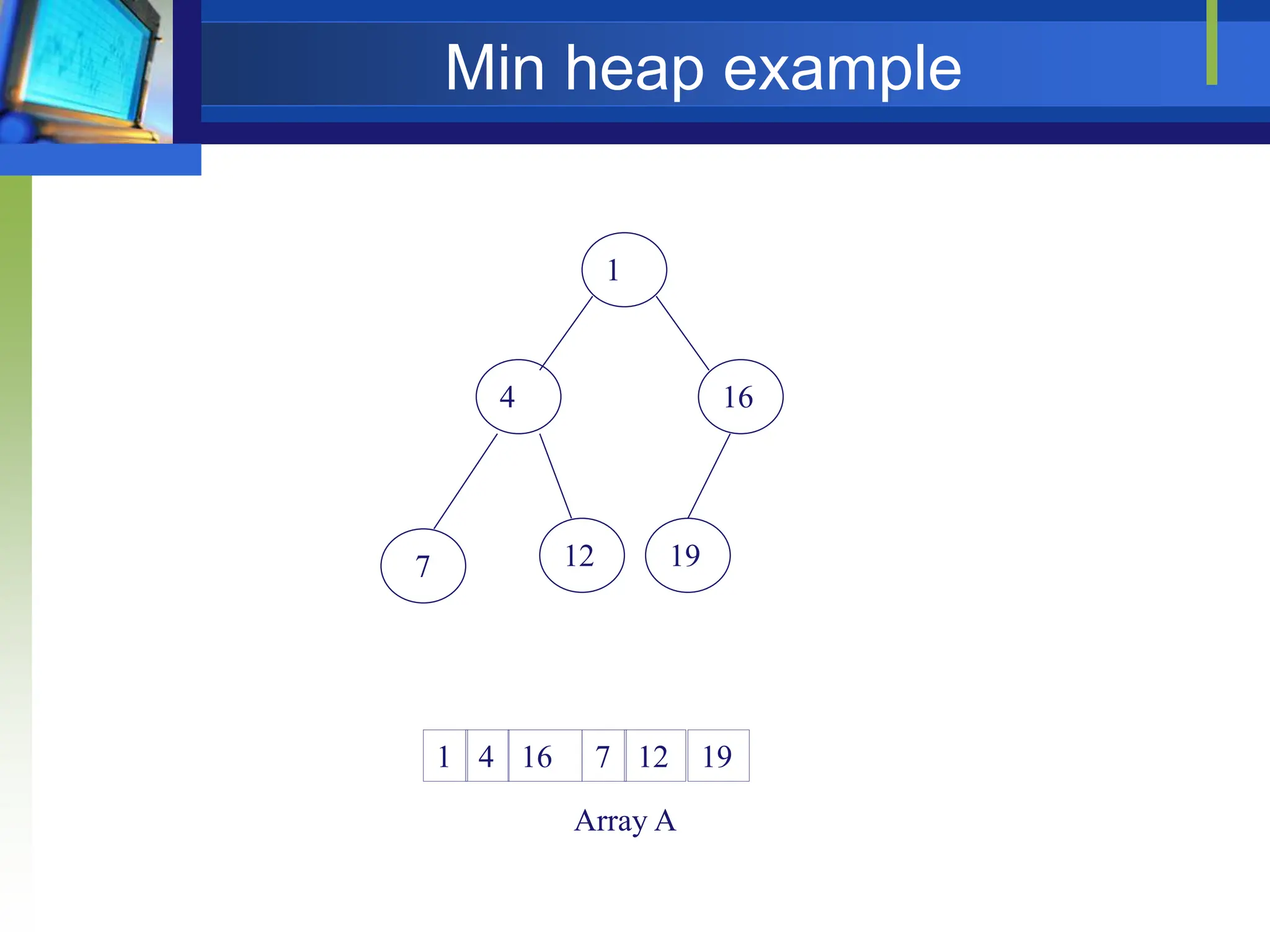
Min Heap
Store data in descending order
Has property of
A[Parent(i)] ≤ A[i]](https://image.slidesharecdn.com/lecture5sortingandorderstatistics-240517091502-73624205/75/Lecture-5_-Sorting-and-order-statistics-pptx-11-2048.jpg)
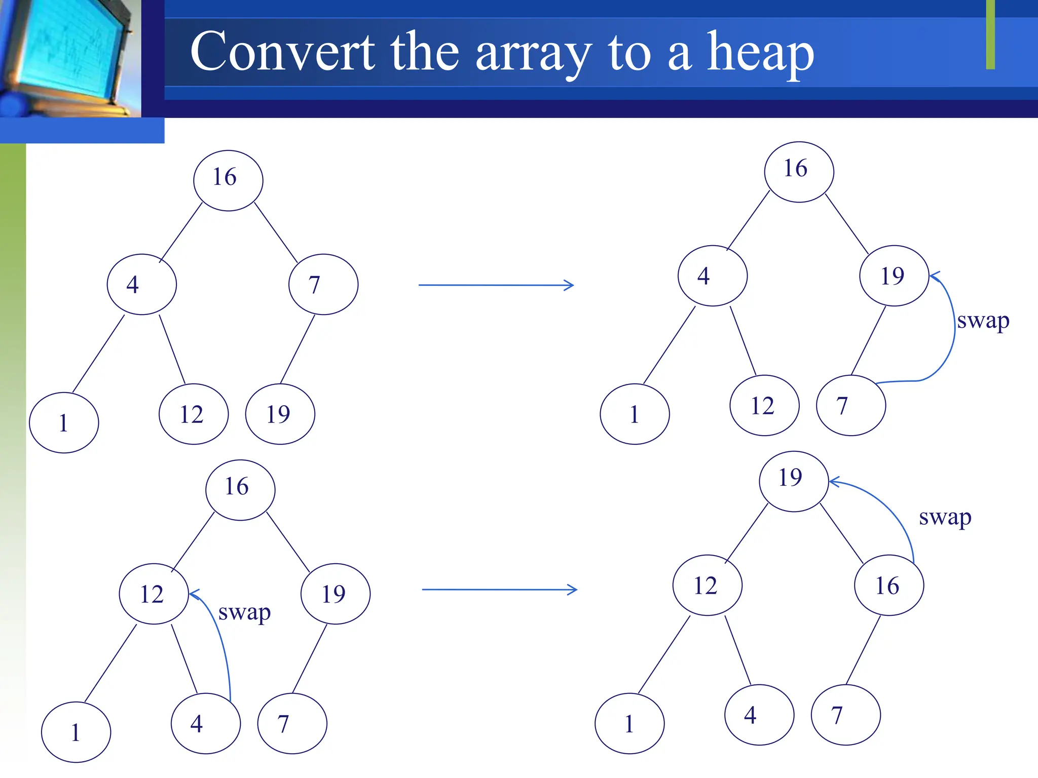
![Heapify
Heapify picks the largest child key and compares it to the parent
key. If parent key is larger then heapify quits, otherwise it swaps
the parent key with the largest child key. So that the parent is
larger than its children.
HEAPIFY (A,i)
p LEFT(i) -- assign left index to p
q RIGHT(i) -- assign right index to q
if p<=heap-size[A] and A[p] > A[i] -- check left child and if larger than parent assign
then largest p -- largest= index of left child
else largest i -- largest= index of parent
if q<=heap-size[A] and A[q] > A[largest] -- check right child and if larger than parent or left child
then largest p -- largest= index of right child
if largest ≠ i -- only swap when parent is less than either child
then exchange A[i] with A[largest]
HEAPIFY (A,largest)](https://image.slidesharecdn.com/lecture5sortingandorderstatistics-240517091502-73624205/75/Lecture-5_-Sorting-and-order-statistics-pptx-15-2048.jpg)
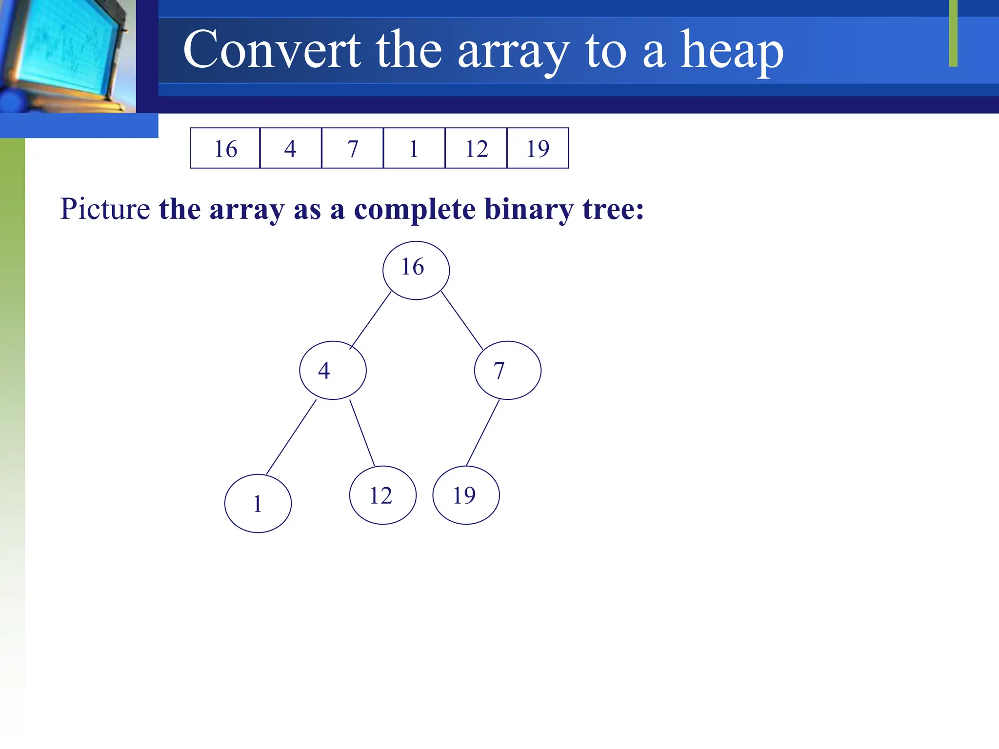
![BUILD HEAP
We can use the procedure 'Heapify' in a bottom-up fashion to convert
an array A[1 . . n] into a heap. Since the elements in the subarray
A[n/2 +1 . . n] are all leaves, the procedure BUILD_HEAP goes
through the remaining nodes of the tree and runs 'Heapify' on each
one. The bottom-up order of processing node guarantees that the
subtree rooted at the children are a heap before 'Heapify' is run at
their parent.
BUILD-HEAP (A)
Heap-size [A] length [A]
for ilength[A/2] to 1
do HEAPIFY (A,i)
Running Time:
Each call to HEAPIFY costs O(lg n)
There are n calls: O(n)
O(n lg n)](https://image.slidesharecdn.com/lecture5sortingandorderstatistics-240517091502-73624205/75/Lecture-5_-Sorting-and-order-statistics-pptx-17-2048.jpg)
![Heap Sort
The heapsort algorithm consists of two phases:
- build a heap from an arbitrary array
- use the heap to sort the data
To sort the elements in the decreasing order, use a min
heap
To sort the elements in the increasing order, use a max heap
HEAPSORT(A)
BUILD-HEAP (A)
for i length[A] down to 2
do exchange A[1] with A[i]
heap-size[A] heap-size[A]-1 --discard node n from heap by
decrementing
HEAPIFY (A,1)](https://image.slidesharecdn.com/lecture5sortingandorderstatistics-240517091502-73624205/75/Lecture-5_-Sorting-and-order-statistics-pptx-27-2048.jpg)
![Heapsort
Given BuildHeap(), an in-place sorting
algorithm is easily constructed:
Maximum element is at A[1]
Discard by swapping with element at A[n]
Decrement heap_size[A]
A[n] now contains correct value
Restore heap property at A[1] by calling
Heapify()
Repeat, always swapping A[1] for
A[heap_size(A)]](https://image.slidesharecdn.com/lecture5sortingandorderstatistics-240517091502-73624205/75/Lecture-5_-Sorting-and-order-statistics-pptx-28-2048.jpg)


![[DSC Europe 25] Boris Perkovic - Lost in performance.pptx](https://cdn.slidesharecdn.com/ss_thumbnails/uq5hrp7vsuahqkxzifux-1-251204082258-fd2ee09d-thumbnail.jpg?width=640&height=640&fit=bounds)
![[DSC Europe 25] Dragana Ilic - AI for Big Data in Astronomy.pptx](https://cdn.slidesharecdn.com/ss_thumbnails/8palya86qaatvjhva1ms-2-dragana-ilic-ai-ilic-251208151906-652b819c-thumbnail.jpg?width=640&height=640&fit=bounds)

![[DSC Europe 25] Vid Stimac - Policy Parsimony: Between Oversimplifying and Ov...](https://cdn.slidesharecdn.com/ss_thumbnails/eqlepagzqp2rhg3gbluh-dsc-stimac-251120-251205090438-059e7f54-thumbnail.jpg?width=640&height=640&fit=bounds)


![[DSC Europe 25] Nikola Rajovic - Hardware Technologies Under the Hood: RISC-V...](https://cdn.slidesharecdn.com/ss_thumbnails/o2gptrmtoyqndgoshwgq-dsc2025-tenstorrent-rajovic-251205090438-814685f5-thumbnail.jpg?width=640&height=640&fit=bounds)

![[DSC Europe 25] Petar Zivanov - AI meets documents From chatbots to AI-powere...](https://cdn.slidesharecdn.com/ss_thumbnails/xer2bb6nrdc8pdpev0pc-8-251204082258-7c2fa4a1-thumbnail.jpg?width=640&height=640&fit=bounds)
![[DSC Europe 25] Bogdan Daniel Maruneac - AI - It starts with you.pptx](https://cdn.slidesharecdn.com/ss_thumbnails/odov3snhrcqs9hx5ny2n-4-251205085715-f1daacfe-thumbnail.jpg?width=640&height=640&fit=bounds)
