The document discusses algorithms for heap data structures and their applications. It begins with an introduction to heaps and their representation as complete binary trees or arrays. It then covers the heap operations of MaxHeapify, building a max heap, and heapsort. Heapsort runs in O(n log n) time by using a max heap to iteratively find and remove the maximum element. The document concludes by discussing how heaps can be used to implement priority queues, with common operations like insert, extract maximum, and increase key running in O(log n) time.

1. Algorithms
Sandeep Kumar Poonia
Head Of Dept. CS/IT
B.E., M.Tech., UGC-NET
LM-IAENG, LM-IACSIT,LM-CSTA, LM-AIRCC, LM-SCIEI, AM-UACEE

2. Algorithms
Introduction to heapsort
Quicksort
Sandeep Kumar Poonia

3. Recap
Asymptotic notation
Merge Sort
Solving Recurrences
The Master Theorem
Sandeep Kumar Poonia

4. Sorting Revisited

So far we’ve talked about two algorithms to
sort an array of numbers



What is the advantage of merge sort?
What is the advantage of insertion sort?
Next on the agenda: Heapsort



Combines advantages of both previous algorithms
Sort in Place – Like insertion sort
O(n Lg n) Worst case – Like Merge sort
Sandeep Kumar Poonia

5. Heaps

A heap can be seen as a complete binary tree:
16
14
10
8
2


7
4
9
1
What makes a binary tree complete?
Is the example above complete?
Sandeep Kumar Poonia
3

6. Heaps

A heap can be seen as a complete binary tree:
16
14
10
8
2

7
4
1
9
1
1
3
1
1
We calls them “nearly complete” binary trees; can
think of unfilled slots as null pointers
Sandeep Kumar Poonia
1

7. Heaps

In practice, heaps are usually implemented as
arrays:
16
14
A = 16 14 10 8
7
9
3
2
4
8
1 =
2
Sandeep Kumar Poonia
10
7
4
1
9
3

8. Heaps

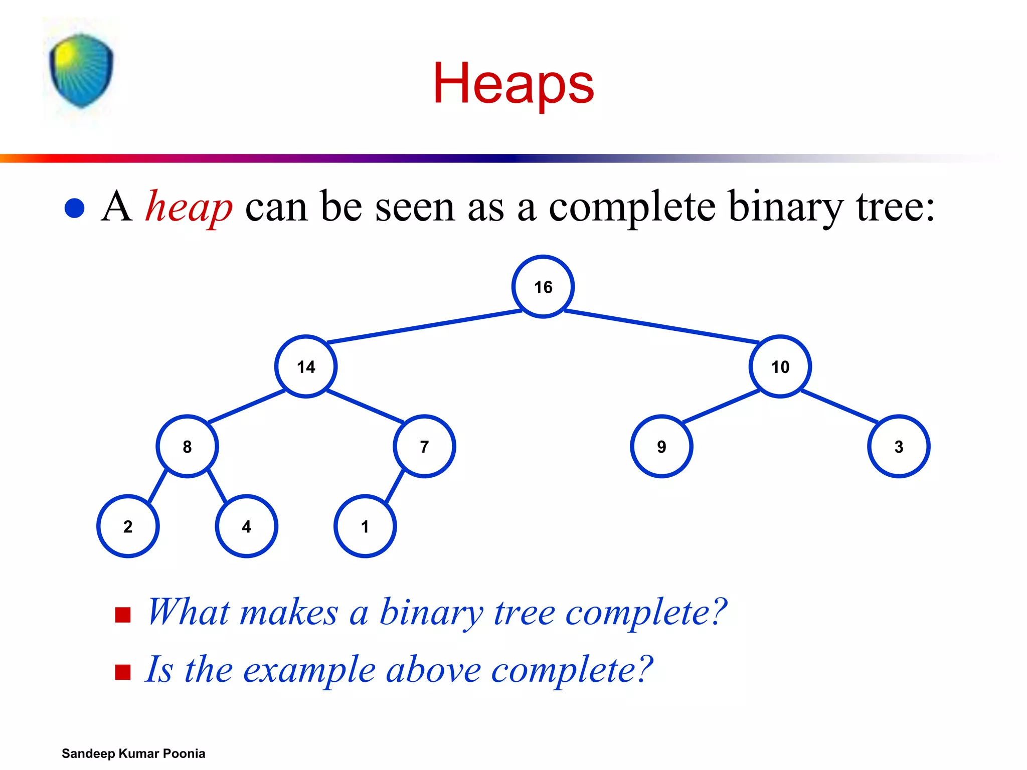
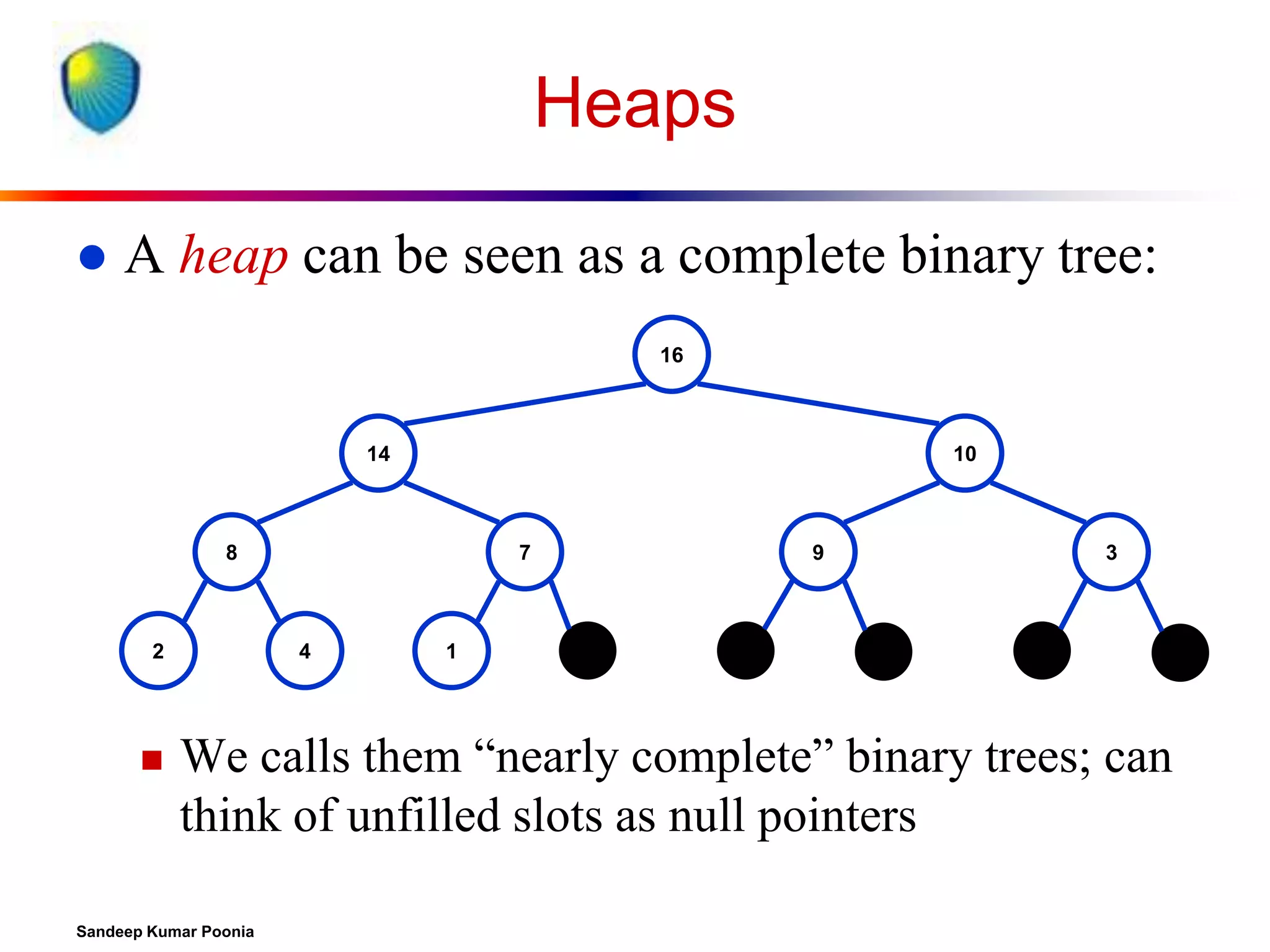
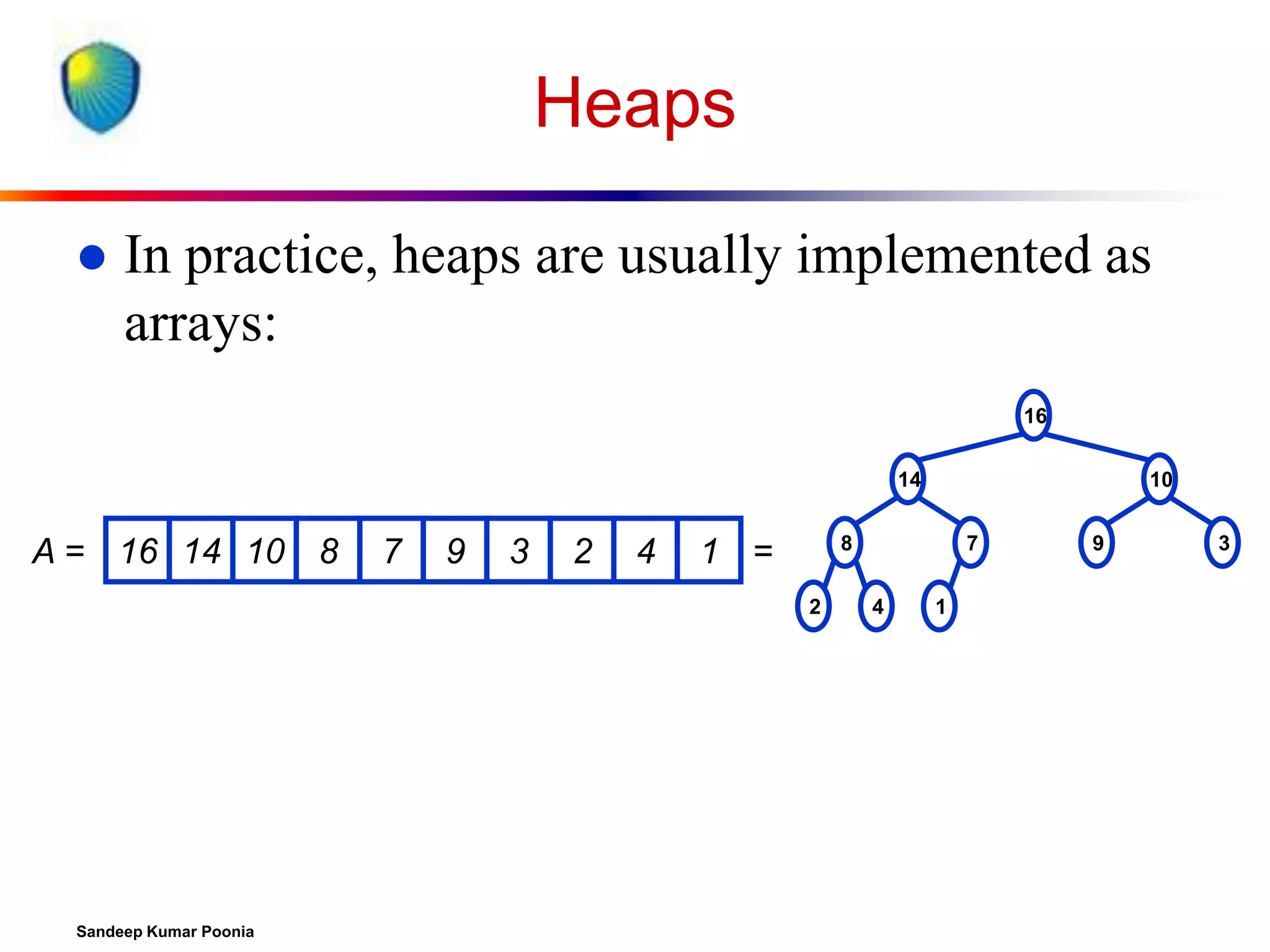
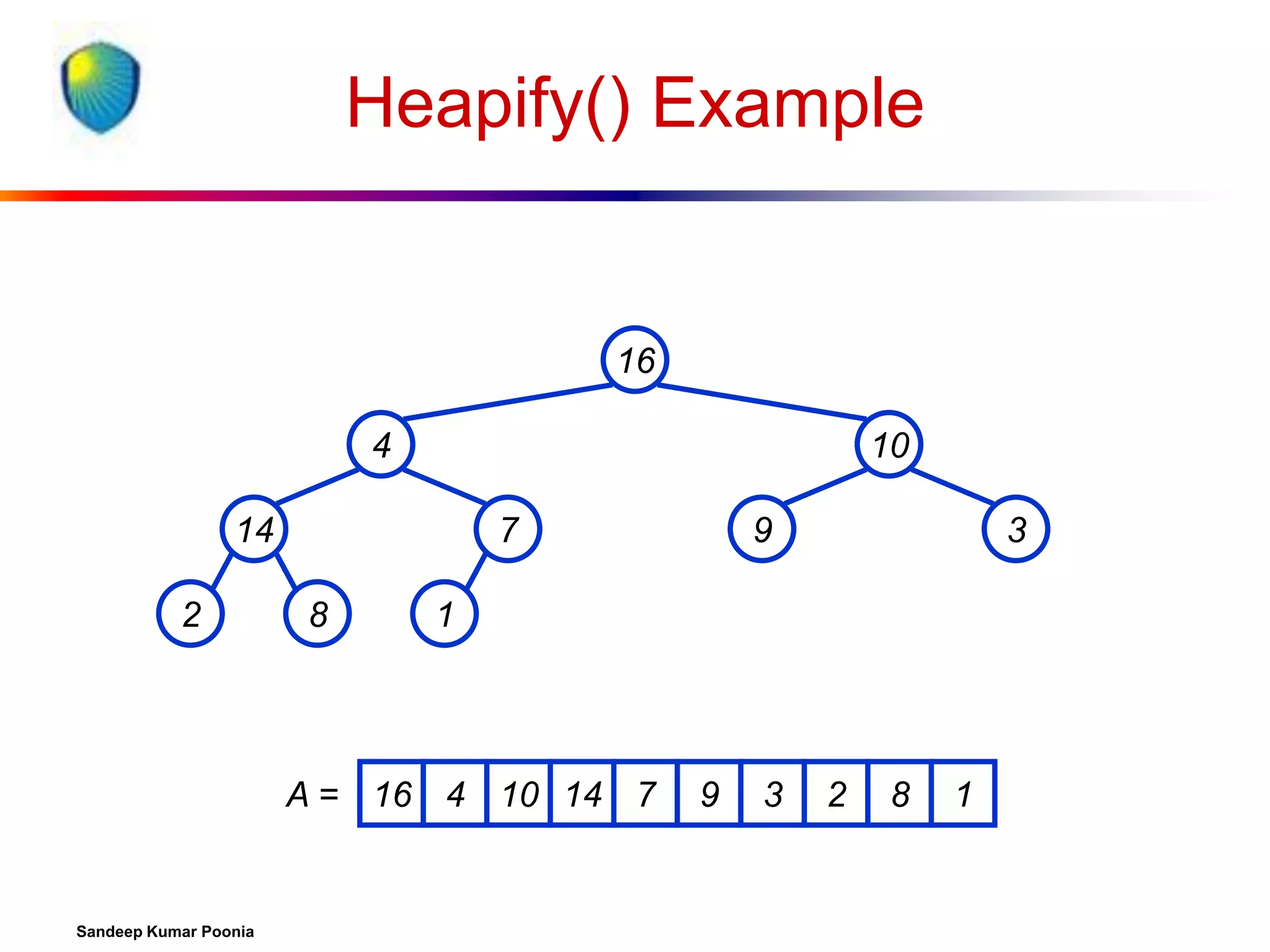
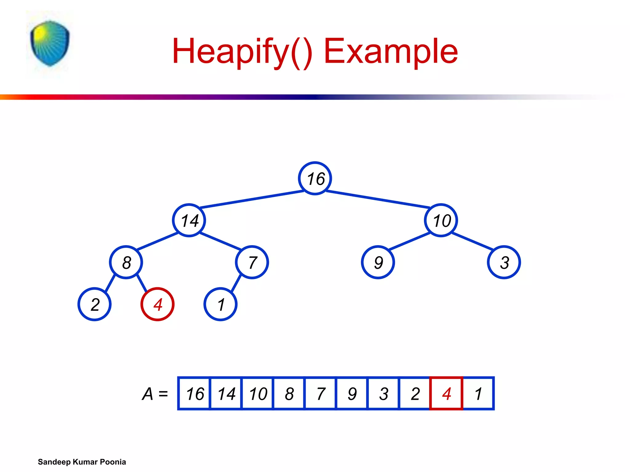
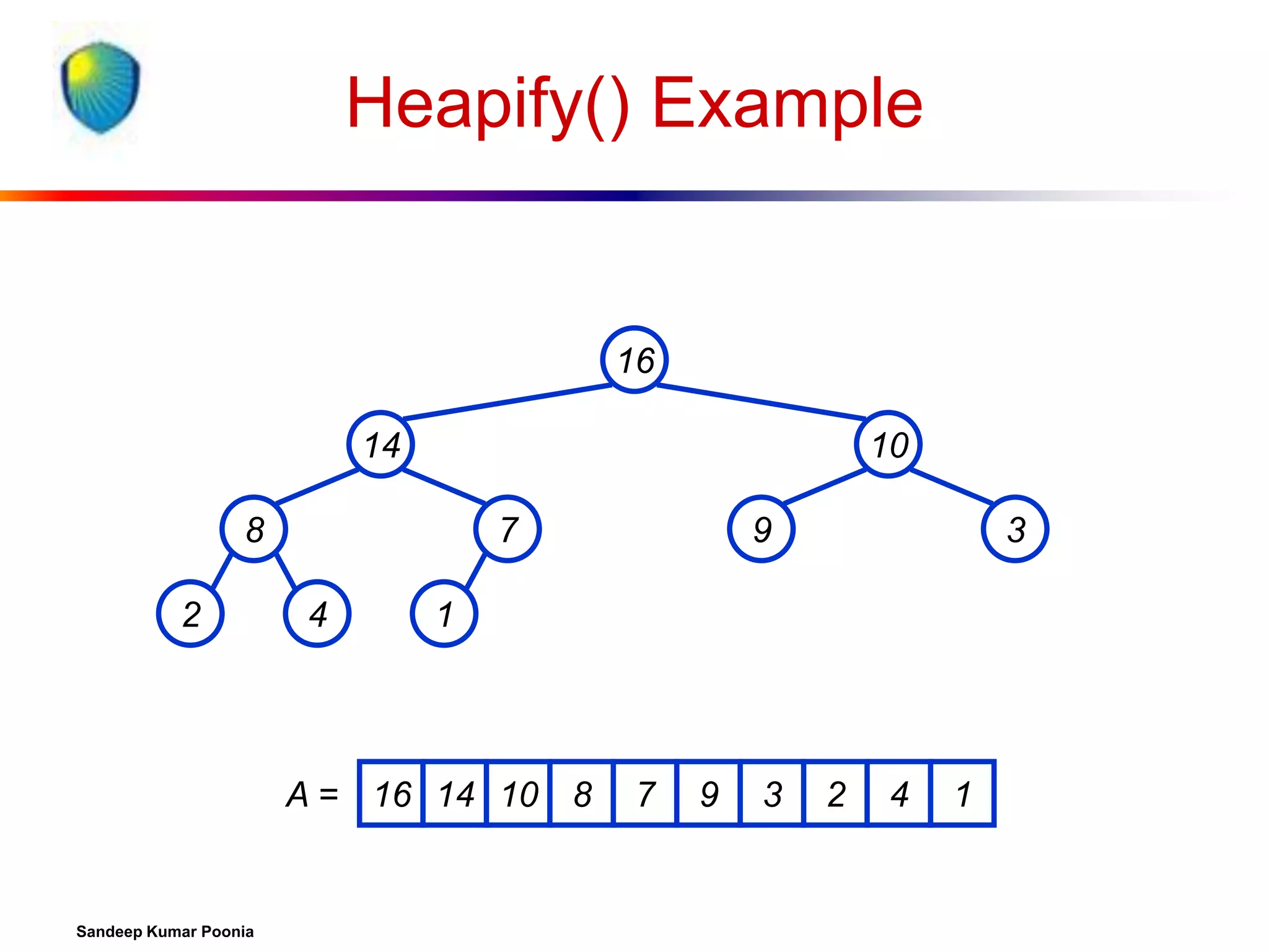
To represent a complete binary tree as an array:





The root node is A[1]
Node i is A[i]
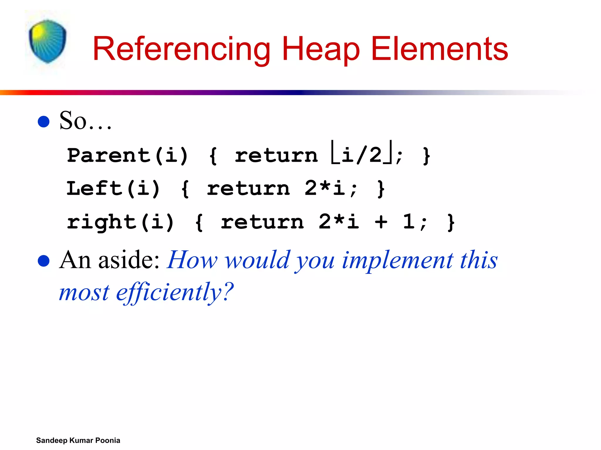
The parent of node i is A[i/2] (note: integer divide)
The left child of node i is A[2i]
The right child of node i is A[2i + 1]
16
14
A = 16 14 10 8
7
9
3
2
4
8
1 =
2
Sandeep Kumar Poonia
10
7
4
1
9
3

9. Referencing Heap Elements

So…
Parent(i) { return i/2; }
Left(i) { return 2*i; }
right(i) { return 2*i + 1; }

An aside: How would you implement this
most efficiently?
Sandeep Kumar Poonia

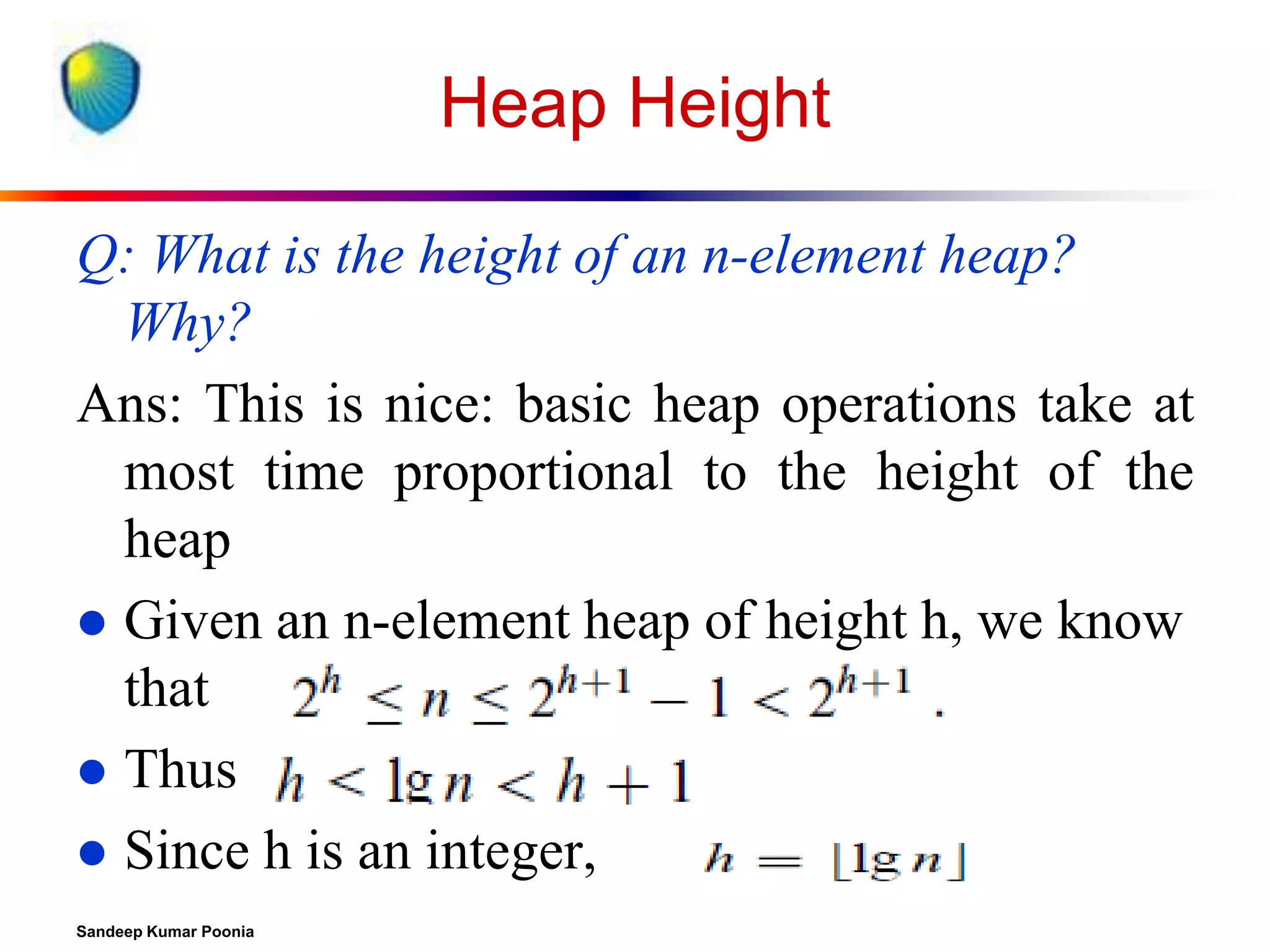
10. The Heap Property

Heaps also satisfy the heap property:
A[Parent(i)]  A[i]
for all nodes i > 1



In other words, the value of a node is at most the
value of its parent
Where is the largest element in a heap stored?
Definitions:


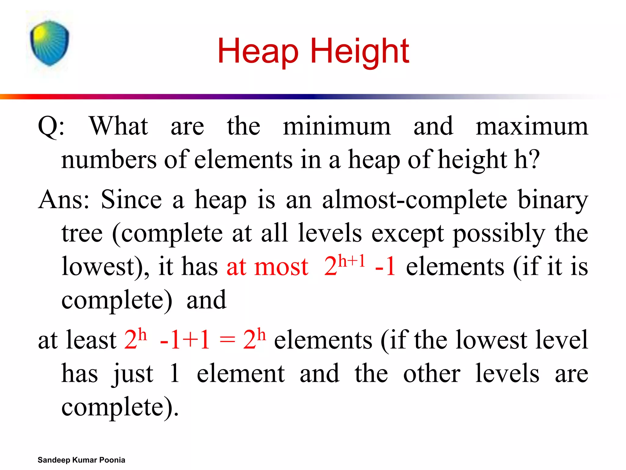
The height of a node in the tree = the number of
edges on the longest downward path to a leaf
The height of a tree = the height of its root
Sandeep Kumar Poonia

11. Heap Height
Q: What are the minimum and maximum
numbers of elements in a heap of height h?
Ans: Since a heap is an almost-complete binary
tree (complete at all levels except possibly the
lowest), it has at most 2h+1 -1 elements (if it is
complete) and
at least 2h -1+1 = 2h elements (if the lowest level
has just 1 element and the other levels are
complete).
Sandeep Kumar Poonia

12. Heap Height
Q: What is the height of an n-element heap?
Why?
Ans: This is nice: basic heap operations take at
most time proportional to the height of the
heap
 Given an n-element heap of height h, we know
that
 Thus
 Since h is an integer,
Sandeep Kumar Poonia

13. Heap Operations: Heapify()

Heapify(): maintain the heap property




Given: a node i in the heap with children l and r
Given: two subtrees rooted at l and r, assumed to
be heaps
Problem: The subtree rooted at i may violate the
heap property.
Action: let the value of the parent node “float
down” so subtree at i satisfies the heap property
 What
do you suppose will be the basic operation
between i, l, and r?
Sandeep Kumar Poonia

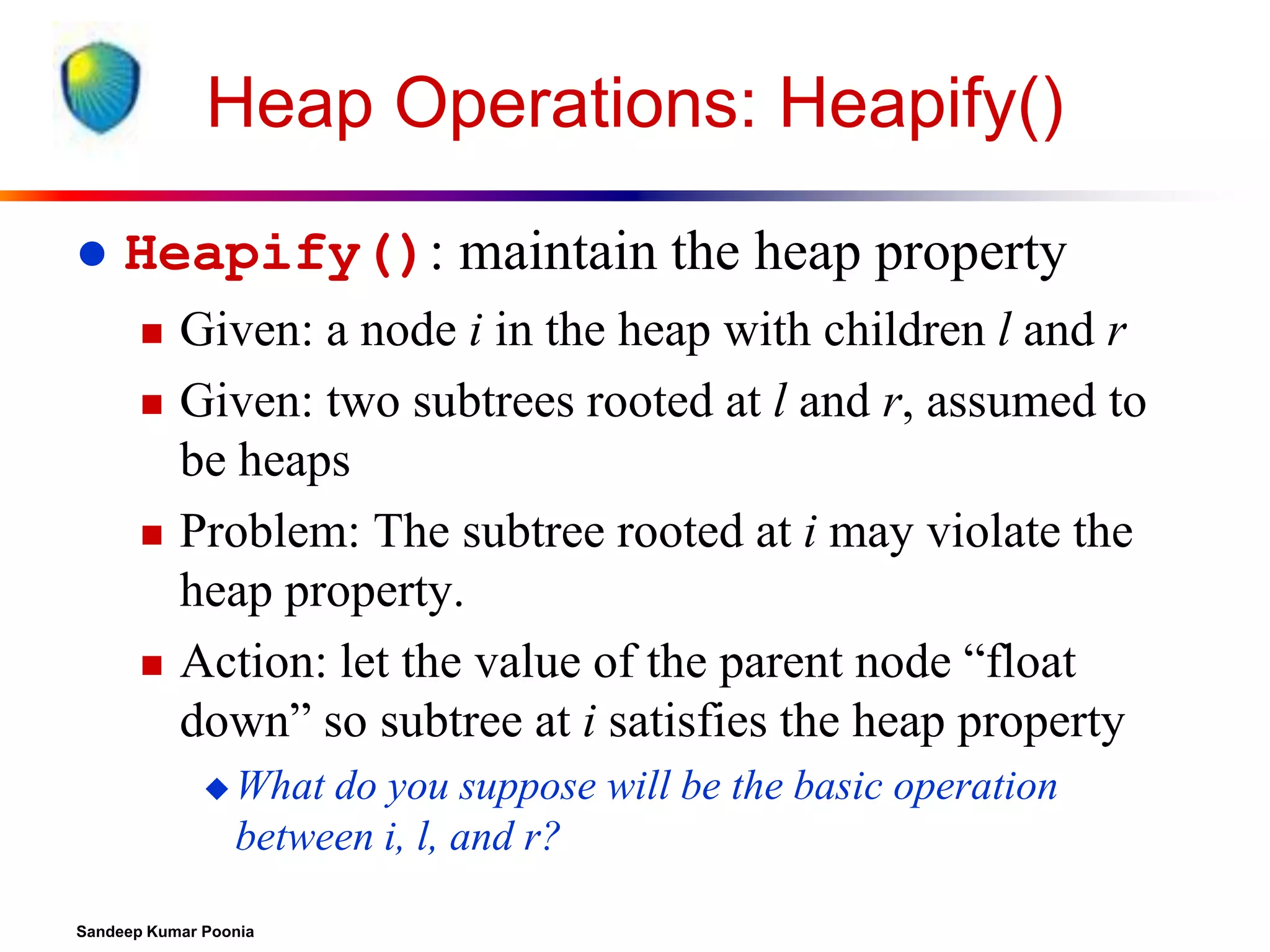
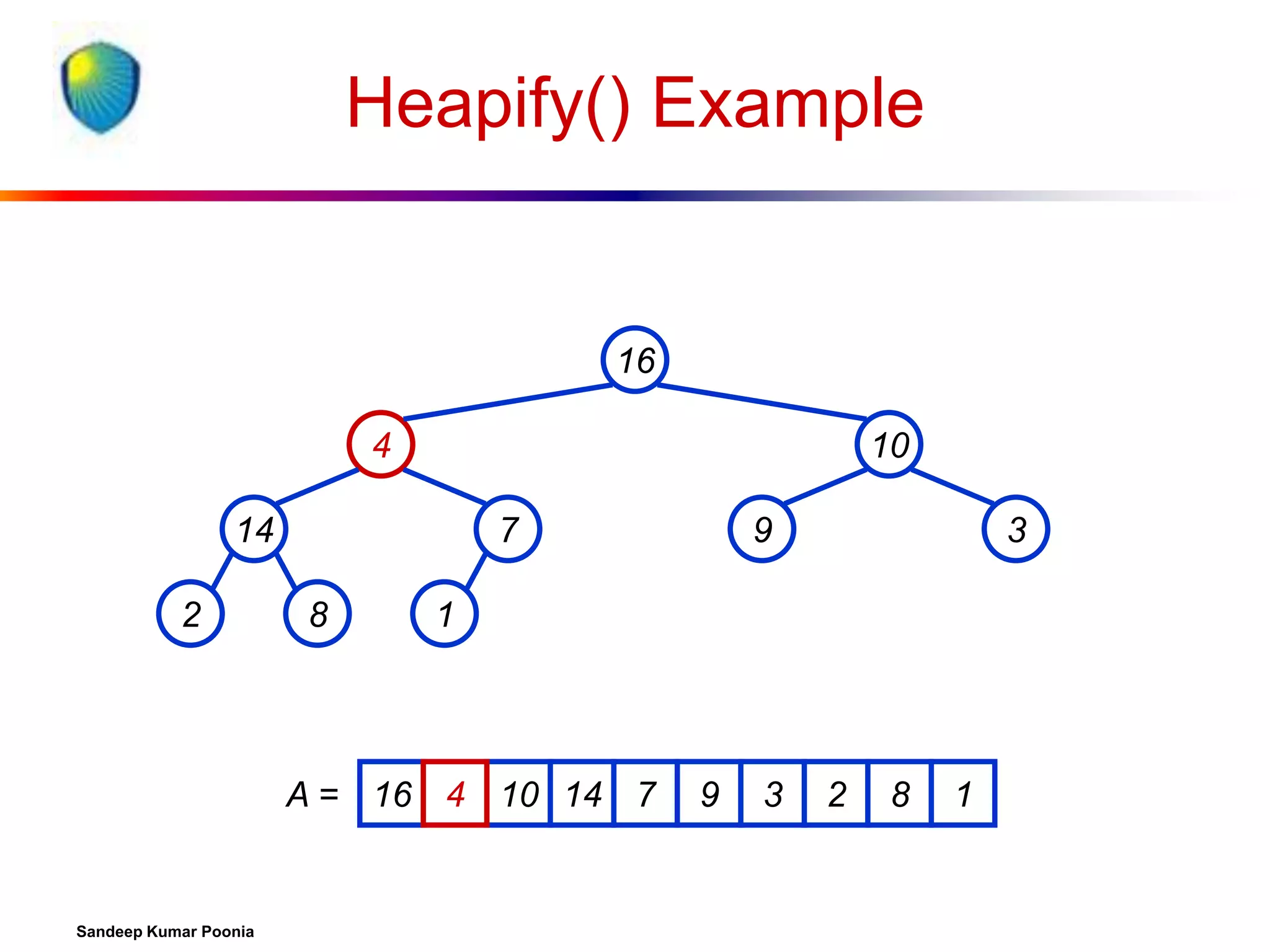
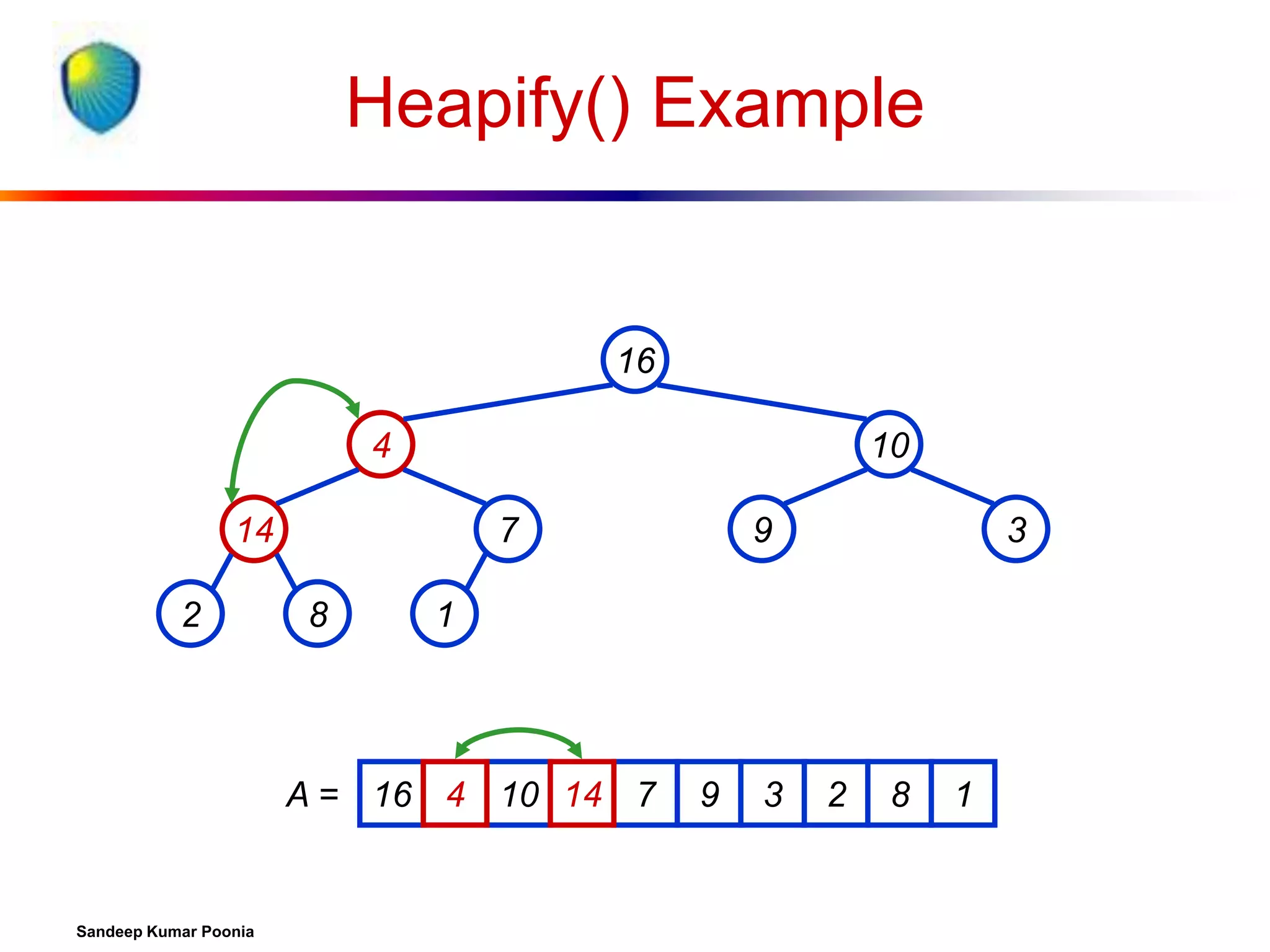
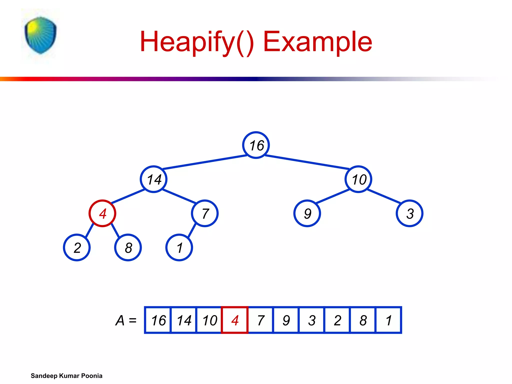
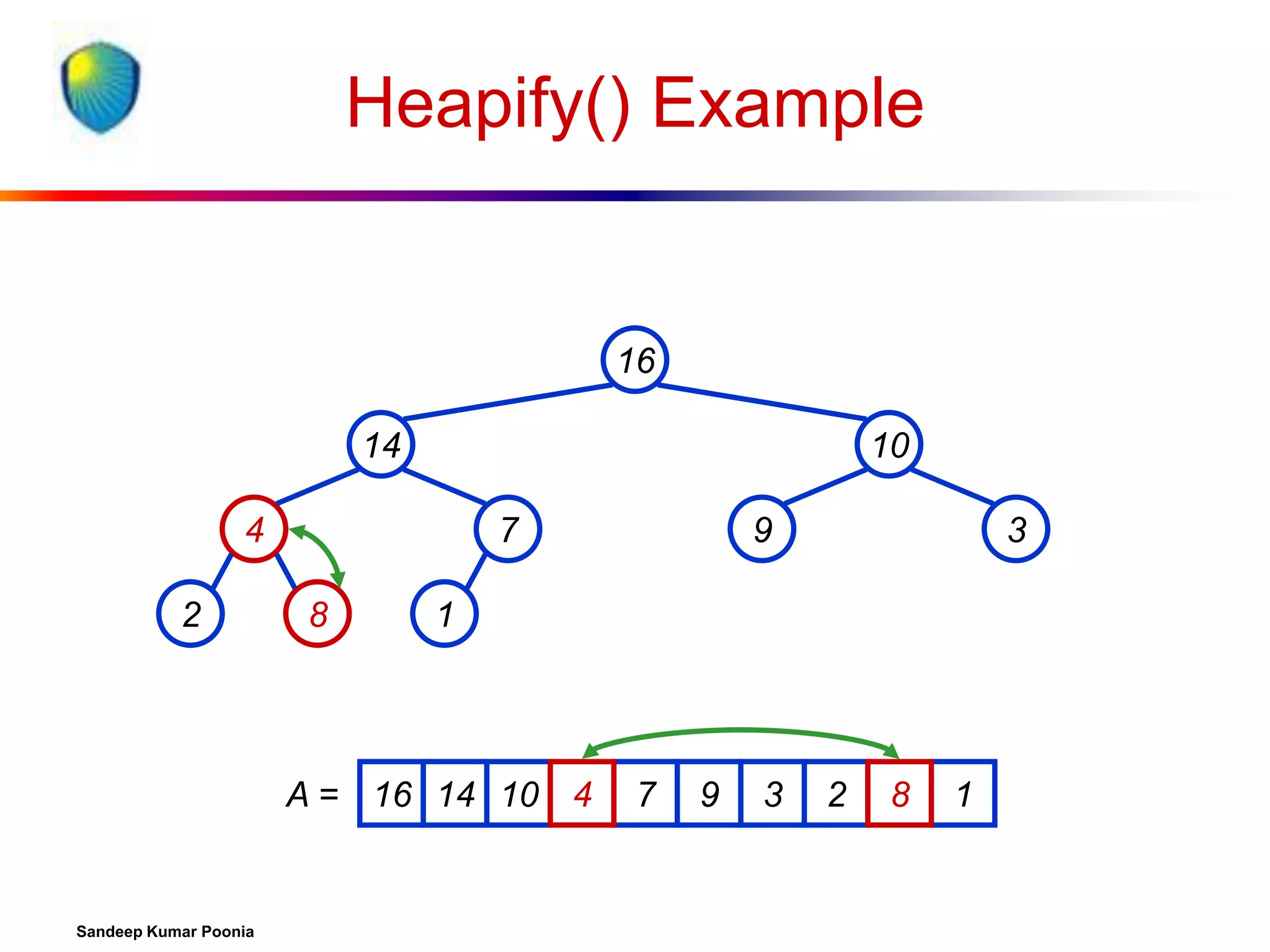
14. Procedure MaxHeapify
MaxHeapify(A, i)
1. l  left(i)
2. r  right(i)
3. if l  heap-size[A] and A[l] > A[i]
4. then largest  l
5. else largest  i
6. if r  heap-size[A] and A[r] > A[largest]
7. then largest  r
8. if largest i
9. then exchange A[i]  A[largest]
10.
MaxHeapify(A, largest)
Sandeep Kumar Poonia
Assumption:
Left(i) and Right(i)
are max-heaps.

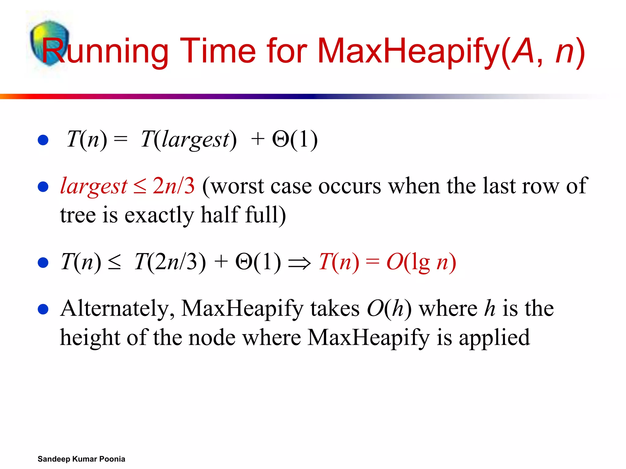
15. Running Time for MaxHeapify
MaxHeapify(A, i)
1. l  left(i)
2. r  right(i)
3. if l  heap-size[A] and A[l] > A[i]
4. then largest  l
5. else largest  i
6. if r  heap-size[A] and A[r] > A[largest]
7. then largest  r
8. if largest i
9. then exchange A[i]  A[largest]
10.
MaxHeapify(A, largest)
Sandeep Kumar Poonia
Time to fix node i
and its children =
(1)
PLUS
Time to fix the
subtree rooted at
one of i’s children =
T(size of subree at
largest)

16. Running Time for MaxHeapify(A, n)

T(n) = T(largest) + (1)

largest  2n/3 (worst case occurs when the last row of
tree is exactly half full)

T(n)  T(2n/3) + (1)  T(n) = O(lg n)

Alternately, MaxHeapify takes O(h) where h is the
height of the node where MaxHeapify is applied
Sandeep Kumar Poonia

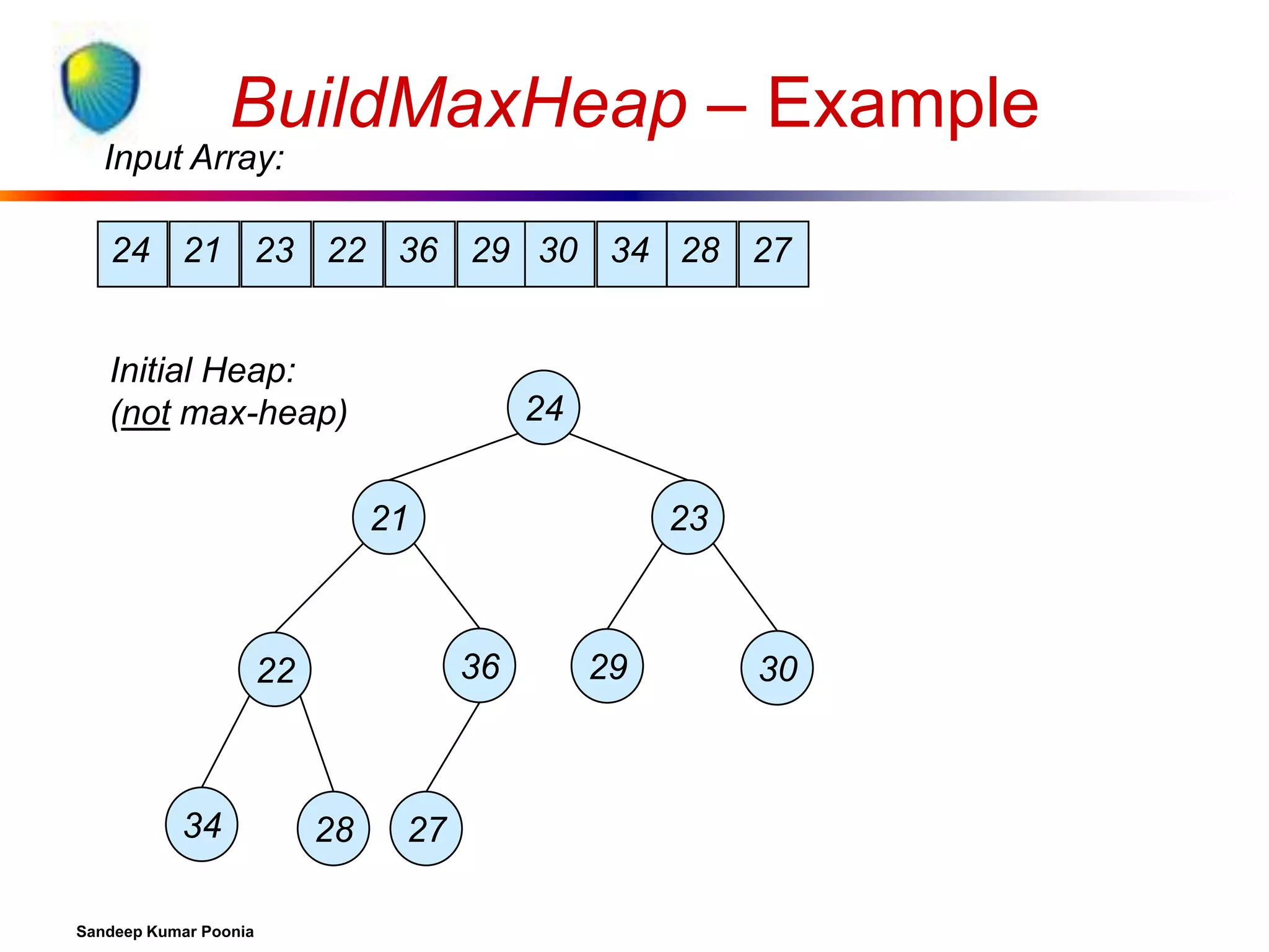
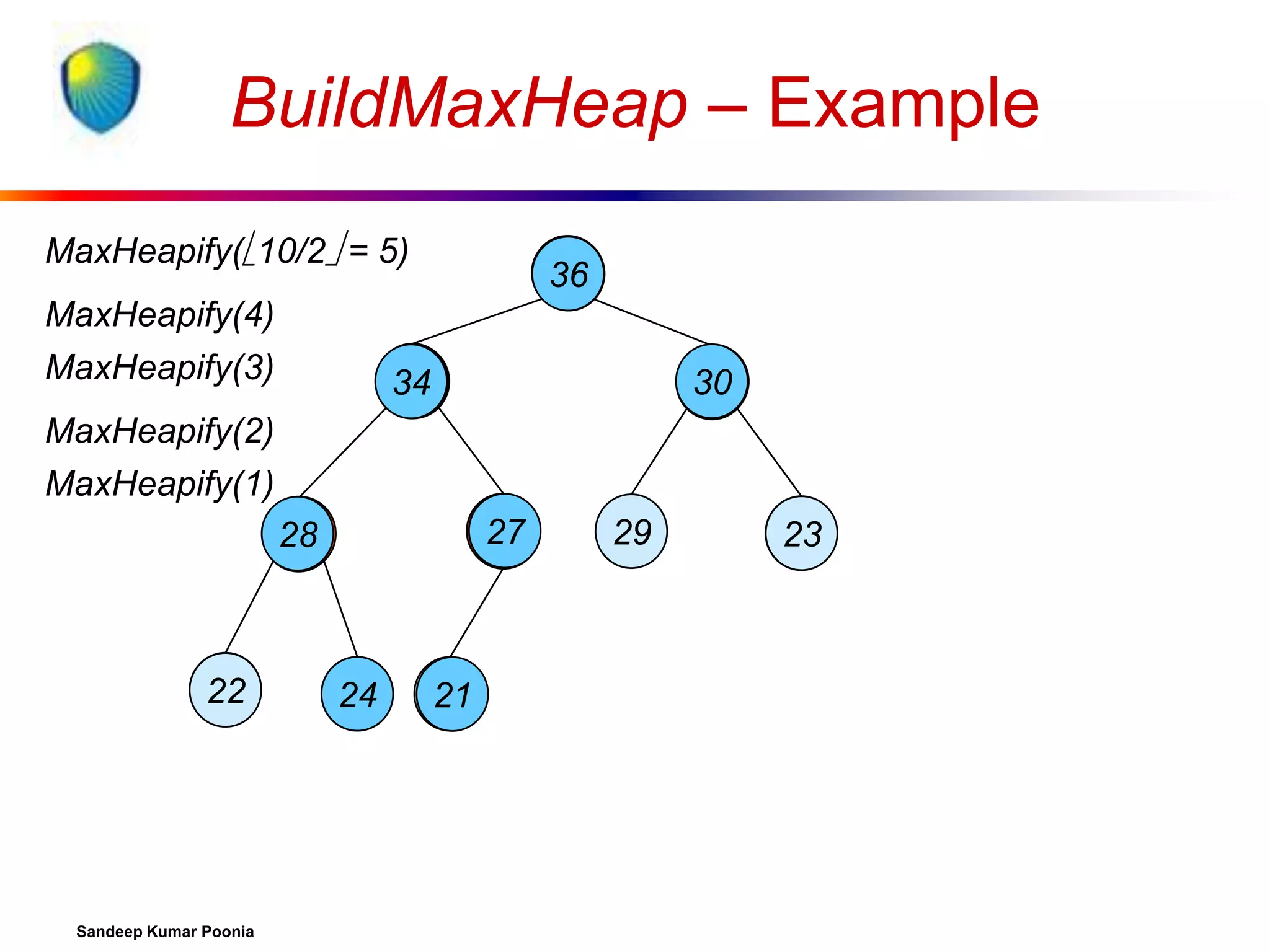
17. Building a heap

Use MaxHeapify to convert an array A into a max-heap.

Call MaxHeapify on each element in a bottom-up
manner.
BuildMaxHeap(A)
1. heap-size[A]  length[A]
2. for i  length[A]/2 downto 1
3.
do MaxHeapify(A, i)
Sandeep Kumar Poonia

18. BuildMaxHeap – Example
Input Array:
24 21 23 22 36 29 30 34 28 27
Initial Heap:
(not max-heap)
24
21
36
22
34
Sandeep Kumar Poonia
23
28
27
29
30

19. BuildMaxHeap – Example
MaxHeapify(10/2 = 5)
MaxHeapify(4)
MaxHeapify(3)
24
36
21
34
24
36
30
23
MaxHeapify(2)
MaxHeapify(1)
36
27
21
28
34
24
22
34
22
Sandeep Kumar Poonia
24
28
27
21
29
30
23

20. Correctness of BuildMaxHeap


Loop Invariant: At the start of each iteration of the for
loop, each node i+1, i+2, …, n is the root of a max-heap.
Initialization:



Before first iteration i = n/2
Nodes n/2+1, n/2+2, …, n are leaves and hence roots of
max-heaps.
Maintenance:



By LI, subtrees at children of node i are max heaps.
Hence, MaxHeapify(i) renders node i a max heap root (while
preserving the max heap root property of higher-numbered
nodes).
Decrementing i reestablishes the loop invariant for the next
iteration.
Sandeep Kumar Poonia

21. Running Time of BuildMaxHeap

Loose upper bound:



Cost of a MaxHeapify call  No. of calls to MaxHeapify
O(lg n)  O(n) = O(nlg n)
Tighter bound:




Cost of a call to MaxHeapify at a node depends on the height,
h, of the node – O(h).
Height of most nodes smaller than n.
Height of nodes h ranges from 0 to lg n.
No. of nodes of height h is n/2h+1
Sandeep Kumar Poonia

22. Heapsort


Sort by maintaining the as yet unsorted elements as a
max-heap.
Start by building a max-heap on all elements in A.


Move the maximum element to its correct final
position.


Decrement heap-size[A].
Restore the max-heap property on A[1..n–1].


Exchange A[1] with A[n].
Discard A[n] – it is now sorted.


Maximum element is in the root, A[1].
Call MaxHeapify(A, 1).
Repeat until heap-size[A] is reduced to 2.
Sandeep Kumar Poonia

23. Heapsort(A)
HeapSort(A)
1. Build-Max-Heap(A)
2. for i  length[A] downto 2
3.
do exchange A[1]  A[i]
4.
heap-size[A]  heap-size[A] – 1
5.
MaxHeapify(A, 1)
Sandeep Kumar Poonia

24. Heapify() Example
16
4
10
14
2
7
8
3
1
A = 16 4 10 14 7
Sandeep Kumar Poonia
9
9
3
2
8
1

25. Heapify() Example
16
4
10
14
2
7
8
3
1
A = 16 4 10 14 7
Sandeep Kumar Poonia
9
9
3
2
8
1

26. Heapify() Example
16
4
10
14
2
7
8
3
1
A = 16 4 10 14 7
Sandeep Kumar Poonia
9
9
3
2
8
1

27. Heapify() Example
16
14
10
4
2
7
8
3
1
A = 16 14 10 4
Sandeep Kumar Poonia
9
7
9
3
2
8
1

28. Heapify() Example
16
14
10
4
2
7
8
3
1
A = 16 14 10 4
Sandeep Kumar Poonia
9
7
9
3
2
8
1

29. Heapify() Example
16
14
10
4
2
7
8
3
1
A = 16 14 10 4
Sandeep Kumar Poonia
9
7
9
3
2
8
1

30. Heapify() Example
16
14
10
8
2
7
4
3
1
A = 16 14 10 8
Sandeep Kumar Poonia
9
7
9
3
2
4
1

31. Heapify() Example
16
14
10
8
2
7
4
3
1
A = 16 14 10 8
Sandeep Kumar Poonia
9
7
9
3
2
4
1

32. Heapify() Example
16
14
10
8
2
7
4
3
1
A = 16 14 10 8
Sandeep Kumar Poonia
9
7
9
3
2
4
1

33. Algorithm Analysis
HeapSort(A)
1. Build-Max-Heap(A)
2. for i  length[A] downto 2
3.
do exchange A[1]  A[i]
4.
heap-size[A]  heap-size[A] – 1
5.
MaxHeapify(A, 1)

In-place

Not Stable

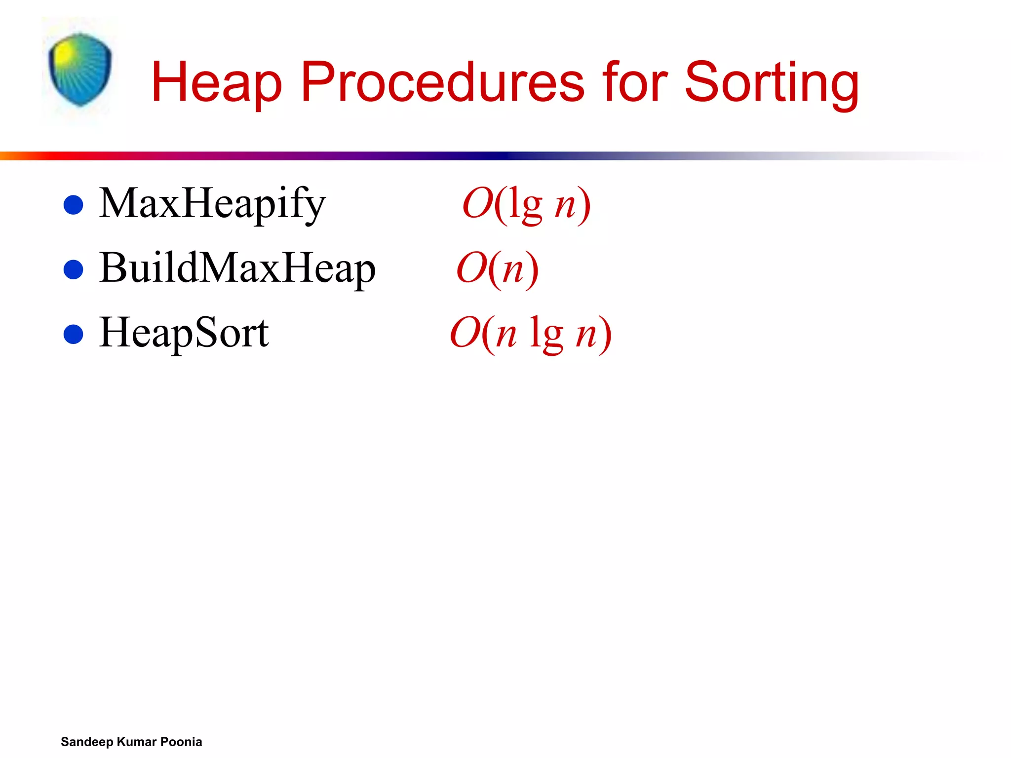
Build-Max-Heap takes O(n) and each of the n-1 calls
to Max-Heapify takes time O(lg n).

Therefore, T(n) = O(n lg n)
Sandeep Kumar Poonia

34. Heap Procedures for Sorting
MaxHeapify
 BuildMaxHeap
 HeapSort

Sandeep Kumar Poonia
O(lg n)
O(n)
O(n lg n)

35. Priority Queue






Popular & important application of heaps.
Max and min priority queues.
Maintains a dynamic set S of elements.
Each set element has a key – an associated value.
Goal is to support insertion and extraction efficiently.
Applications:


Ready list of processes in operating systems by their
priorities – the list is highly dynamic
In event-driven simulators to maintain the list of events to be
simulated in order of their time of occurrence.
Sandeep Kumar Poonia

36. Basic Operations

Operations on a max-priority queue:

Insert(S, x) - inserts the element x into the set S






S  S  {x}.
Maximum(S) - returns the element of S with the largest
key.
Extract-Max(S) - removes and returns the element of S with
the largest key.
Increase-Key(S, x, k) – increases the value of element x’s
key to the new value k.
Min-priority queue supports Insert, Minimum,
Extract-Min, and Decrease-Key.
Heap gives a good compromise between fast insertion
but slow extraction and vice versa.
Sandeep Kumar Poonia

37. Heap Property (Max and Min)

Max-Heap

For every node excluding the root,
value is at most that of its parent: A[parent[i]]  A[i]

Largest element is stored at the root.
In any subtree, no values are larger than the value
stored at subtree root.

Min-Heap




For every node excluding the root,
value is at least that of its parent: A[parent[i]]  A[i]
Smallest element is stored at the root.
In any subtree, no values are smaller than the value
stored at subtree root
Sandeep Kumar Poonia

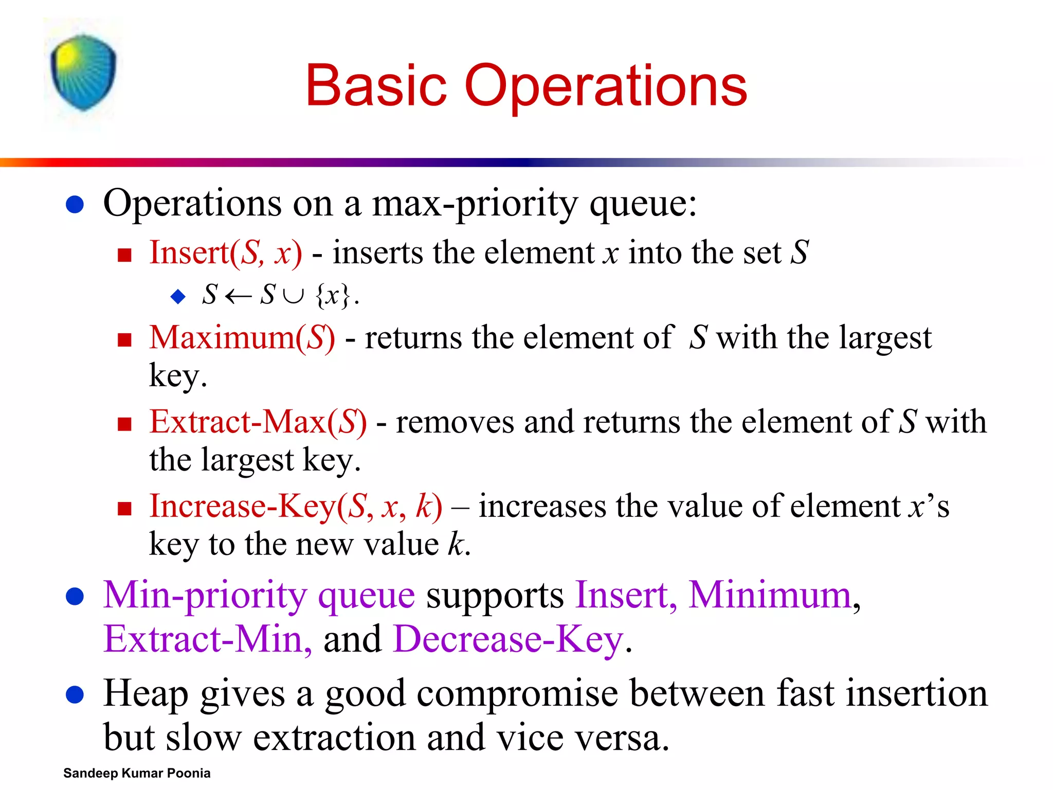
38. Heap-Extract-Max(A)
Implements the Extract-Max operation.
Heap-Extract-Max(A,n)
1. if n < 1
2. then error “heap underflow”
3. max  A[1]
4. A[1]  A[n]
5. n  n - 1
6. MaxHeapify(A, 1)
7. return max
Running time : Dominated by the running time of MaxHeapify
= O(lg n)
Sandeep Kumar Poonia

39. Heap-Insert(A, key)
Heap-Insert(A, key)
1. heap-size[A]  heap-size[A] + 1
2.
i  heap-size[A]
4. while i > 1 and A[Parent(i)] < key
5.
do A[i]  A[Parent(i)]
6.
i  Parent(i)
7. A[i]  key
Running time is O(lg n)
The path traced from the new leaf to the root has
length O(lg n)
Sandeep Kumar Poonia

40. Heap-Increase-Key(A, i, key)
Heap-Increase-Key(A, i, key)
1
If key < A[i]
2
then error “new key is smaller than the current key”
3 A[i]  key
4
while i > 1 and A[Parent[i]] < A[i]
5
do exchange A[i]  A[Parent[i]]
6
i  Parent[i]
Heap-Insert(A, key)
1
heap-size[A]  heap-size[A] + 1
2 A[heap-size[A]]  –
3
Heap-Increase-Key(A, heap-size[A], key)
Sandeep Kumar Poonia

41. Quicksort
Sorts in place
 Sorts O(n lg n) in the average case
 Sorts O(n2) in the worst case
 So why would people use it instead of merge
sort?

Sandeep Kumar Poonia

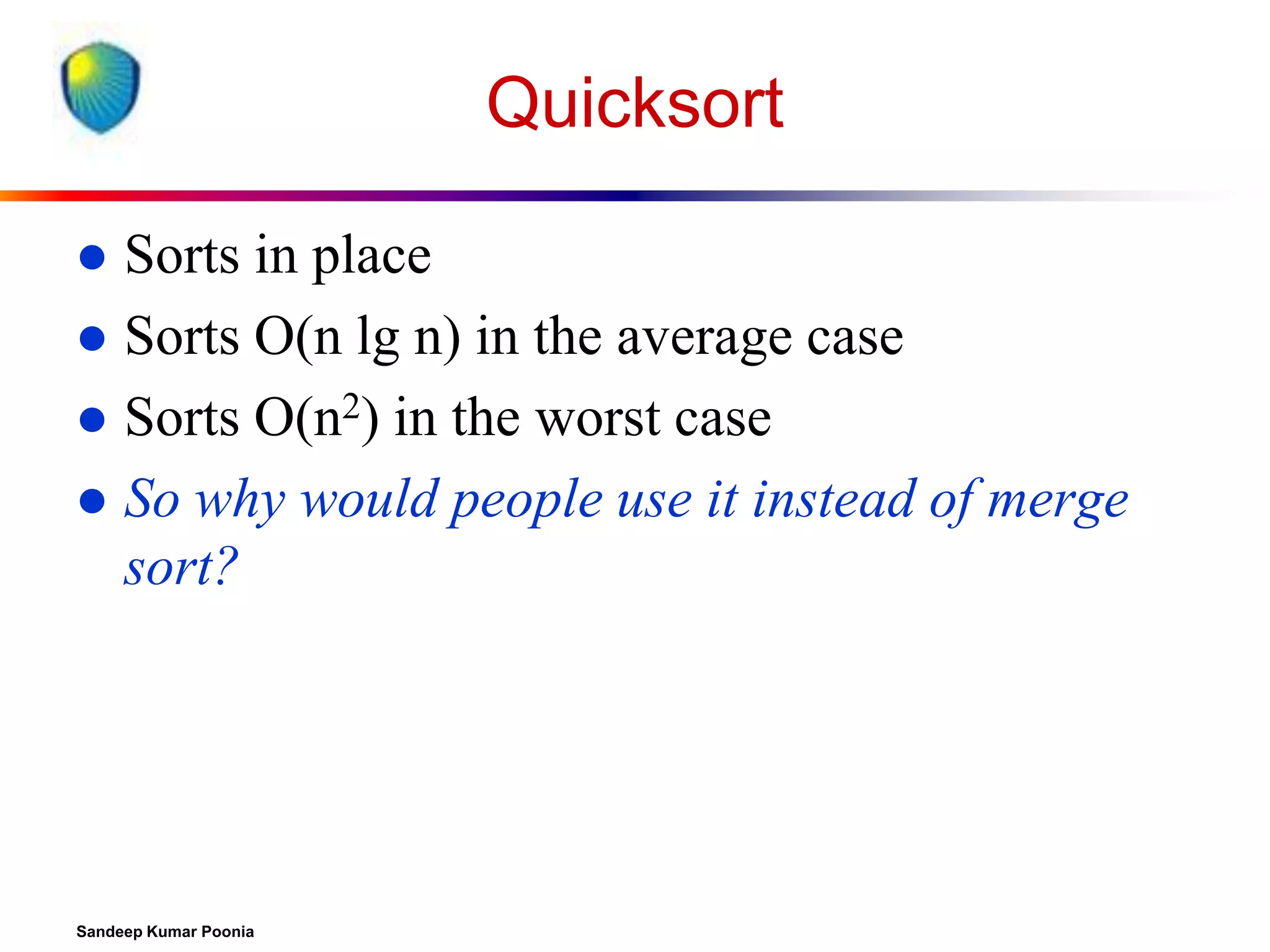
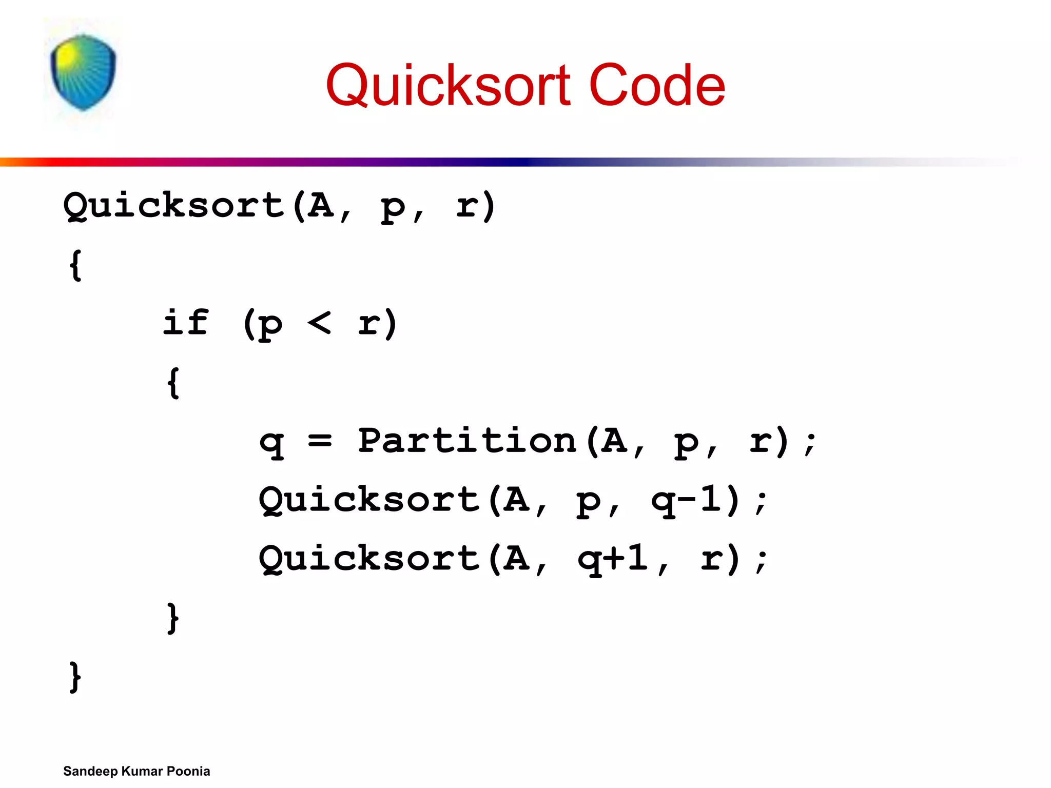
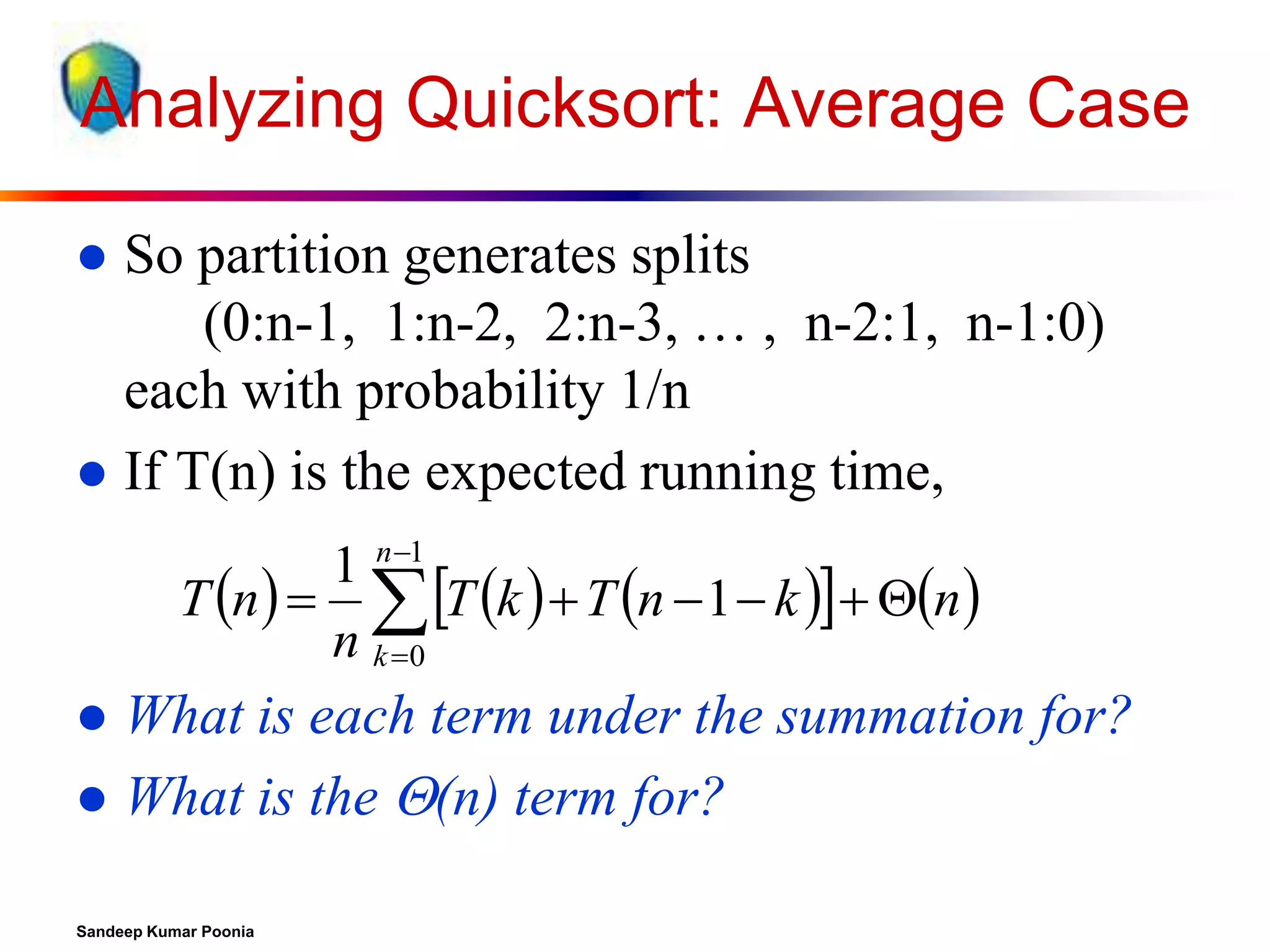
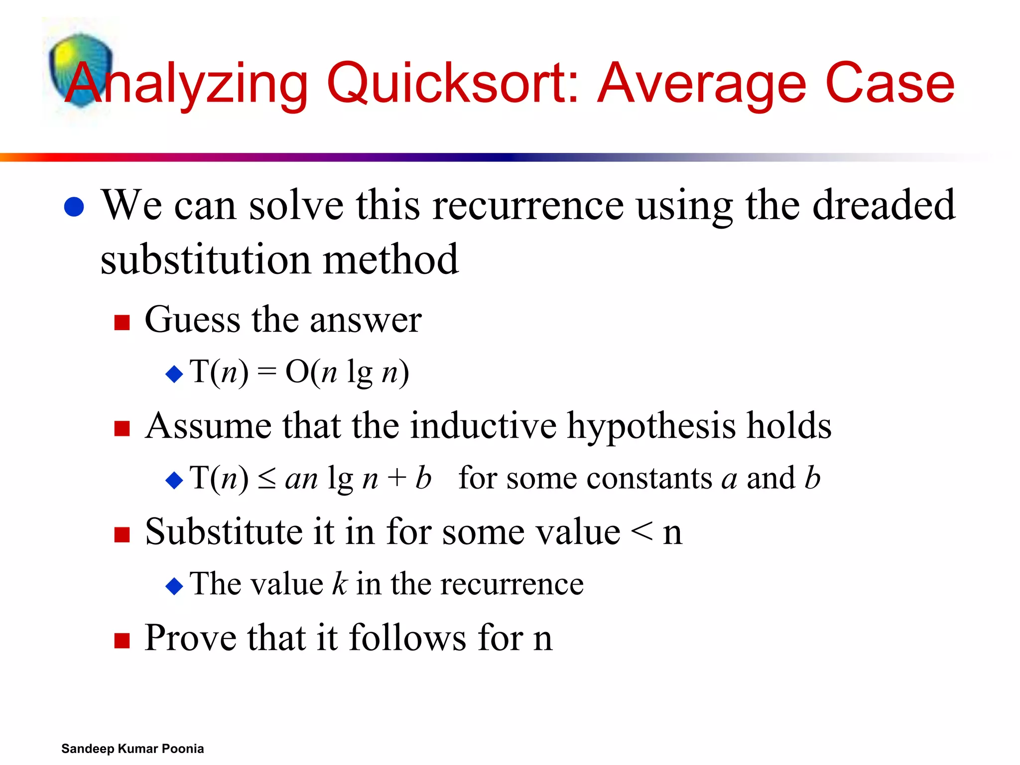
42. Quicksort

Another divide-and-conquer algorithm

The array A[p..r] is partitioned into two nonempty subarrays A[p..q] and A[q+1..r]
 Invariant:
All elements in A[p..q] are less than all
elements in A[q+1..r]


The subarrays are recursively sorted by calls to
quicksort
Unlike merge sort, no combining step: two
subarrays form an already-sorted array
Sandeep Kumar Poonia

43. Quicksort Code
Quicksort(A, p, r)
{
if (p < r)
{
q = Partition(A, p, r);
Quicksort(A, p, q-1);
Quicksort(A, q+1, r);
}
}
Sandeep Kumar Poonia

44. Partition

Clearly, all the action takes place in the
partition() function


Rearranges the subarray in place
End result:
 Two
subarrays
 All values in first subarray  all values in second


Returns the index of the “pivot” element
separating the two subarrays
How do you suppose we implement this
function?
Sandeep Kumar Poonia

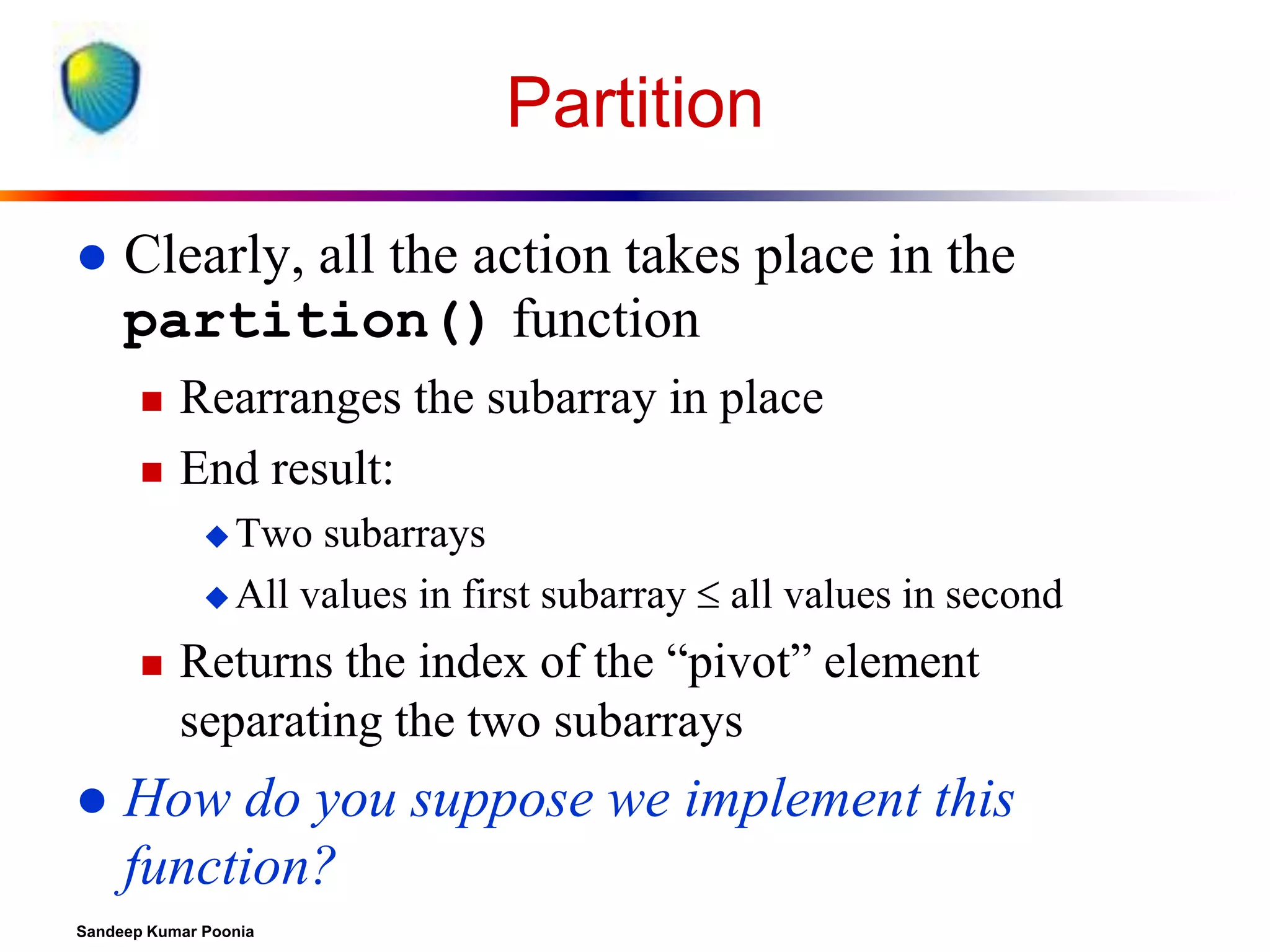
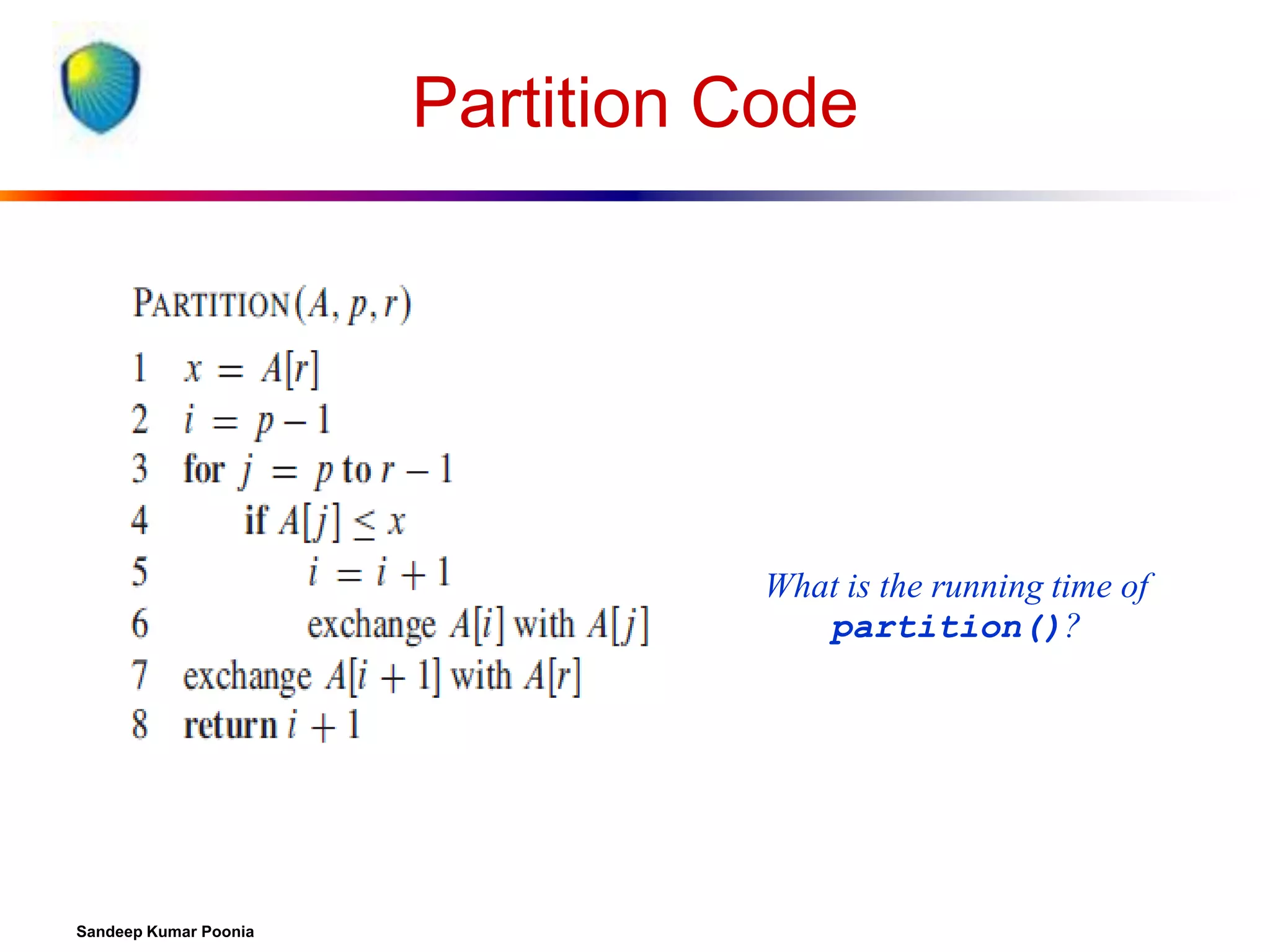
45. Partition In Words

Partition(A, p, r):


Select an element to act as the “pivot” (which?)
Grow two regions, A[p..i] and A[j..r]
 All
elements in A[p..i] <= pivot
 All elements in A[j..r] >= pivot





Increment i until A[i] >= pivot
Decrement j until A[j] <= pivot
Swap A[i] and A[j]
Repeat until i >= j
Return j
Sandeep Kumar Poonia

46. Partition Code
What is the running time of
partition()?
Sandeep Kumar Poonia

47. Review: Analyzing Quicksort

What will be the worst case for the algorithm?


What will be the best case for the algorithm?


Partition is balanced
Which is more likely?


Partition is always unbalanced
The latter, by far, except...
Will any particular input elicit the worst case?

Yes: Already-sorted input
Sandeep Kumar Poonia

48. Review: Analyzing Quicksort

In the worst case: one subarray have 0 element
and another n-1 elements
T(1) = (1)
T(n) = T(n - 1) + (n)

Works out to
T(n) = (n2)
Sandeep Kumar Poonia

49. Review: Analyzing Quicksort

In the best case: each has <= n/2 elements
T(n) = 2T(n/2) + (n)

What does this work out to?
T(n) = (n lg n)
Sandeep Kumar Poonia

50. Review: Analyzing Quicksort
(Average Case)

Intuitively, a real-life run of quicksort will
produce a mix of “bad” and “good” splits



Randomly distributed among the recursion tree
Pretend for intuition that they alternate between
best-case (n/2 : n/2) and worst-case (n-1 : 1)
What happens if we bad-split root node, then
good-split the resulting size (n-1) node?
Sandeep Kumar Poonia

51. Review: Analyzing Quicksort
(Average Case)

Intuitively, a real-life run of quicksort will
produce a mix of “bad” and “good” splits



Randomly distributed among the recursion tree
Pretend for intuition that they alternate between
best-case (n/2 : n/2) and worst-case (n-1 : 1)
What happens if we bad-split root node, then
good-split the resulting size (n-1) node?
 We
end up with three subarrays, size 1, (n-1)/2, (n-1)/2
 Combined cost of splits = n + n -1 = 2n -1 = O(n)
 No worse than if we had good-split the root node!
Sandeep Kumar Poonia

52. Review: Analyzing Quicksort
(Average Case)
Intuitively, the O(n) cost of a bad split
(or 2 or 3 bad splits) can be absorbed
into the O(n) cost of each good split
 Thus running time of alternating bad and good
splits is still O(n lg n), with slightly higher
constants

Sandeep Kumar Poonia

53. Analyzing Quicksort: Average Case

For simplicity, assume:


All inputs distinct (no repeats)
Slightly different partition() procedure
 partition
around a random element, which is not
included in subarrays
 all splits (0:n-1, 1:n-2, 2:n-3, … , n-1:0) equally likely
What is the probability of a particular split
happening?
 Answer: 1/n

Sandeep Kumar Poonia

54. Analyzing Quicksort: Average Case
So partition generates splits
(0:n-1, 1:n-2, 2:n-3, … , n-2:1, n-1:0)
each with probability 1/n
 If T(n) is the expected running time,

1 n1
T n    T k   T n  1  k   n 
n k 0
What is each term under the summation for?
 What is the (n) term for?

Sandeep Kumar Poonia

55. Analyzing Quicksort: Average Case

So…
1 n 1
T n    T k   T n  1  k   n 
n k 0
2 n 1
  T k   n 
n k 0
Sandeep Kumar Poonia
Write it on
the board

56. Analyzing Quicksort: Average Case

We can solve this recurrence using the
substitution method




Guess the answer
Assume that the inductive hypothesis holds
Substitute it in for some value < n
Prove that it follows for n
Sandeep Kumar Poonia

57. Analyzing Quicksort: Average Case

We can solve this recurrence using the
substitution method

Guess the answer
 What’s



the answer?
Assume that the inductive hypothesis holds
Substitute it in for some value < n
Prove that it follows for n
Sandeep Kumar Poonia

58. Analyzing Quicksort: Average Case

We can solve this recurrence using the dreaded
substitution method

Guess the answer
 T(n)



= O(n lg n)
Assume that the inductive hypothesis holds
Substitute it in for some value < n
Prove that it follows for n
Sandeep Kumar Poonia

59. Analyzing Quicksort: Average Case

We can solve this recurrence using the dreaded
substitution method

Guess the answer
 T(n)

= O(n lg n)
Assume that the inductive hypothesis holds
 What’s


the inductive hypothesis?
Substitute it in for some value < n
Prove that it follows for n
Sandeep Kumar Poonia

60. Analyzing Quicksort: Average Case

We can solve this recurrence using the dreaded
substitution method

Guess the answer
 T(n)

Assume that the inductive hypothesis holds
 T(n)


= O(n lg n)
 an lg n + b for some constants a and b
Substitute it in for some value < n
Prove that it follows for n
Sandeep Kumar Poonia

61. Analyzing Quicksort: Average Case

We can solve this recurrence using the dreaded
substitution method

Guess the answer
 T(n)

Assume that the inductive hypothesis holds
 T(n)

= O(n lg n)
 an lg n + b for some constants a and b
Substitute it in for some value < n
 What

value?
Prove that it follows for n
Sandeep Kumar Poonia

62. Analyzing Quicksort: Average Case

We can solve this recurrence using the dreaded
substitution method

Guess the answer
 T(n)

Assume that the inductive hypothesis holds
 T(n)

 an lg n + b for some constants a and b
Substitute it in for some value < n
 The

= O(n lg n)
value k in the recurrence
Prove that it follows for n
Sandeep Kumar Poonia

63. Analyzing Quicksort: Average Case

We can solve this recurrence using the dreaded
substitution method

Guess the answer
 T(n)

Assume that the inductive hypothesis holds
 T(n)

 an lg n + b for some constants a and b
Substitute it in for some value < n
 The

= O(n lg n)
value k in the recurrence
Prove that it follows for n
 Grind
Sandeep Kumar Poonia
through it…

64. Analyzing Quicksort: Average Case
2 n 1
T n    T k   n 
n k 0
2 n 1
  ak lg k  b   n 
n k 0
The recurrence to be solved
Plug in inductive hypothesis
What are we doing here?
2  n 1

What are we doing here?
 b   ak lg k  b   n  Expand out the k=0 case
n  k 1

2 n 1
2b
  ak lg k  b  
 n 
n k 1
n
2b/n is just a constant,
What are we doing here?
so fold it into (n)
2 n 1
  ak lg k  b   n 
n k 1
Note: leaving the same
recurrence as the book
Sandeep Kumar Poonia

65. Analyzing Quicksort: Average Case
2 n 1
T n    ak lg k  b   n 
n k 1
2 n 1
2 n 1
  ak lg k   b  n 
n k 1
n k 1
The recurrence to be solved
Distribute the summation
What are we doing here?
2a n 1
2b
the summation:

k lg k  (n  1)  n  Evaluateare we doing here?
What

b+b+…+b = b (n-1)
n k 1
n
2a n 1

 k lg k  2b  n 
n k 1
This summation gets its own set of slides later
Sandeep Kumar Poonia
Since n-1<n,we doing here?
What are 2b(n-1)/n < 2b

66. Analyzing Quicksort: Average Case
2a n 1
T n  
 k lg k  2b  n 
n k 1




The recurrence to be solved
2a  1 2
1 2
We’ll prove this
 n lg n  n   2b  n  What the hell? later
n 2
8 
a
an lg n  n  2b  n 
Distribute the (2a/n) term
What are we doing here?
4
a  Remember, our goal is to get

an lg n  b   n   b  n 
What are we doing here?
T(n)  an lg n + b
4 

Pick a large enough that
an lg n  b
How did we do this?
an/4 dominates (n)+b
Sandeep Kumar Poonia

67. Analyzing Quicksort: Average Case

So T(n)  an lg n + b for certain a and b



Thus the induction holds
Thus T(n) = O(n lg n)
Thus quicksort runs in O(n lg n) time on average
Sandeep Kumar Poonia