1. Data Analysis & Forecasting Faculty of Development Economics
TIME SERIES ANALYSIS
BOUNDS TEST FOR COINTEGRATION WITHIN ARDL
MODELLING APPROACH
Another way to test for cointegration and causality is the Bounds Test for Cointegration
within ARDL modelling approach. This model was developed by Pesaran et al. (2001) and
can be applied irrespective of the order of integration of the variables (irrespective of
whether regressors are purely I (0), purely I (1) or mutually cointegrated). This is specially
linked with the ECM models and called VECM.
1. THE MODEL
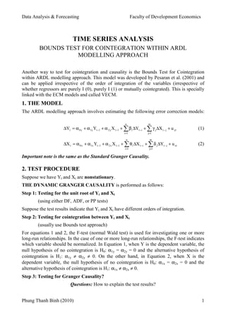
The ARDL modelling approach involves estimating the following error correction models:
n m
∆Yt = α 0 y + α 1y Yt −1 + α 2 y X t −1 + ∑ β i ∆Yt −i + ∑ γ j ∆X t − j + u yt (1)
i =1 j=1
n m
∆X t = α 0 x + α1x Yt −1 + α 2 x X t −1 + ∑ θ i ∆X t −i + ∑ δ j ∆Yt − j + u xt (2)
i =1 j=1
Important note is the same as the Standard Granger Causality.
2. TEST PROCEDURE
Suppose we have Yt and Xt are nonstationary.
THE DYNAMIC GRANGER CAUSALITY is performed as follows:
Step 1: Testing for the unit root of Yt and Xt
(using either DF, ADF, or PP tests)
Suppose the test results indicate that Yt and Xt have different orders of integration.
Step 2: Testing for cointegration between Yt and Xt
(usually use Bounds test approach)
For equations 1 and 2, the F-test (normal Wald test) is used for investigating one or more
long-run relationships. In the case of one or more long-run relationships, the F-test indicates
which variable should be normalized. In Equation 1, when Y is the dependent variable, the
null hypothesis of no cointegration is H0: α1y = α2y = 0 and the alternative hypothesis of
cointegration is H1: α1y ≠ α2y ≠ 0. On the other hand, in Equation 2, when X is the
dependent variable, the null hypothesis of no cointegration is H0: α1x = α2x = 0 and the
alternative hypothesis of cointegration is H1: α1x ≠ α2x ≠ 0.
Step 3: Testing for Granger Causality?
Questions: How to explain the test results?
Phung Thanh Binh (2010) 1