This document provides an overview of Bernoulli statistics and distributions, including key concepts like Bernoulli trials, the Bernoulli distribution, and the mean and variance of Bernoulli random variables. It also discusses the binomial distribution and how it arises from a series of independent Bernoulli trials. Finally, it covers the Poisson distribution and how it can model the number of events occurring in a fixed interval of time or space given a constant average rate of occurrence.


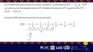
![To find the expected value E[X], we use the formula:
Where represents each possible outcome, and P(X= ) is the
probability of obtaining outcome .](https://image.slidesharecdn.com/bernoulli-binomial-poisson-and-rvs-240414071153-816391f4/85/Theory-of-Probability-Bernoulli-Binomial-Passion-41-320.jpg)